PDF Run this chapter's code LaTeX source Comments
Chapter 11Learning With Errors (LWE)
11.1From exact linear algebra to a noisy problem#
Solving a system of linear equations over a field is one of the oldest solved problems in mathematics. Given \(\mathbf{A}\in\mathbb{Z}_q^{m\times n}\) and \(\mathbf{b}\in\mathbb{Z}_q^{m}\), Gaussian elimination recovers \(\mathbf{s}\) from \(\mathbf{A}\mathbf{s}=\mathbf{b}\) when \(\mathbf{A}\) has full column rank and the system is consistent. Its usual cost is \(O(mn^2)\) field operations (or \(O(n^3)\) for a square \(n\times n\) system). Because the problem is this easy, an exact full-rank linear system carries no cryptographic hardness: an adversary can recover the secret directly.
The Learning With Errors (LWE) problem, introduced by Regev [1], makes a single, deliberate change to this picture: it perturbs each equation by a small additive error. The observed system is \[\mathbf{b} = \mathbf{A}\mathbf{s} + \mathbf{e} \pmod q,\] where \(\mathbf{e}\) is a short noise vector drawn from a prescribed distribution. Ordinary exact elimination no longer solves this noisy modular system: it can detect inconsistency, but it does not identify the planted secret. LWE hardness is a parameterized cryptographic assumption about recovering that secret from many finite-modulus, small-error samples; it is not a claim that every noisy regression problem is hard. This chapter develops LWE as a formal object: its distribution, its two decision problems, the geometry that explains its hardness, and the worst-case reduction that makes it a trustworthy foundation. It is the assumption on which ML-KEM (Chapter 16) and ML-DSA (Chapter 17) ultimately rest.
11.2The LWE distribution#
Throughout, fix a dimension \(n\) (the security parameter), a modulus \(q=q(n)\), and an error distribution \(\chi\) over \(\mathbb{Z}_q\) concentrated on values of small absolute value. Vectors are column vectors, and \(\langle\cdot,\cdot\rangle\) denotes the inner product modulo \(q\).
Definition 11.1 (LWE distribution). For a fixed secret \(\mathbf{s}\in\mathbb{Z}_q^{n}\), the LWE distribution \(A_{\mathbf{s},\chi}\) over \(\mathbb{Z}_q^{n}\times\mathbb{Z}_q\) is sampled by drawing \(\mathbf{a}\leftarrow\mathbb{Z}_q^{n}\) uniformly and \(e\leftarrow\chi\), and outputting \[(\mathbf{a},\,b), \qquad b=\langle \mathbf{a},\mathbf{s}\rangle + e \pmod q.\]
Collecting \(m\) independent samples and stacking the vectors \(\mathbf{a}_i\) as the rows of a matrix \(\mathbf{A}\in\mathbb{Z}_q^{m\times n}\) gives the compact matrix form \[(\mathbf{A},\,\mathbf{b}), \qquad \mathbf{b}=\mathbf{A}\mathbf{s}+\mathbf{e}\pmod q,\quad \mathbf{e}\leftarrow\chi^{m}.\] The name is now transparent: the adversary is asked to learn the hidden \(\mathbf{s}\) from many noisy linear measurements of it. The only obstruction is the error \(\mathbf{e}\); without it the samples are an exactly solvable system.
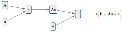
Remark 1.1 (On the secret distribution). The definition draws \(\mathbf{s}\) uniformly from \(\mathbb{Z}_q^{n}\), but a standard transformation puts LWE into normal form, in which the secret is drawn from the error distribution \(\chi\) and is therefore itself short, without loss of hardness. Deployed schemes exploit this: in ML-KEM the secret is a small vector sampled from a centered binomial distribution (Chapter 15), which shortens keys and speeds arithmetic while preserving security.
11.3The two LWE problems#
LWE gives rise to a search problem and a decision problem, and the distinction is central: encryption schemes are proved secure against the decision version, while the search version is the more intuitive statement of “recover the key.”
Definition 11.2 (Search-LWE). Given \(m\) independent samples \((\mathbf{A},\mathbf{b})\) drawn from \(A_{\mathbf{s},\chi}\) for a fixed but unknown \(\mathbf{s}\in\mathbb{Z}_q^{n}\), recover \(\mathbf{s}\).
Definition 11.3 (Decision-LWE). Distinguish, with non-negligible advantage, between the two distributions on \(\mathbb{Z}_q^{m\times n}\times\mathbb{Z}_q^{m}\):
the LWE distribution: \((\mathbf{A},\mathbf{A}\mathbf{s}+\mathbf{e})\) with \(\mathbf{s}\leftarrow\mathbb{Z}_q^{n}\) and \(\mathbf{e}\leftarrow\chi^{m}\);
the uniform distribution: \((\mathbf{A},\mathbf{u})\) with \(\mathbf{u}\leftarrow\mathbb{Z}_q^{m}\) uniform and independent of \(\mathbf{A}\).
The decision formulation is what makes LWE a workhorse for cryptography: if LWE samples are computationally indistinguishable from uniform randomness, then a ciphertext that masks a message by adding it to an LWE sample is indistinguishable from a random string, which is exactly semantic security. Remarkably, the two problems are equivalent.
Proposition 11.4 (Search–decision equivalence). For a prime modulus \(q=\mathrm{poly}(n)\), Search-LWE and Decision-LWE are equivalent up to a polynomial factor in running time and sample complexity: an efficient algorithm for either yields an efficient algorithm for the other.
The forward direction (search solves decision) is immediate. The reverse – bootstrapping a mere distinguisher into a full secret-recovery algorithm – is the substantial part: one guesses each coordinate \(s_j\in\mathbb{Z}_q\) in turn, uses the distinguisher to test the guess, and amplifies. Regev proved the equivalence for prime \(q=\mathrm{poly}(n)\) [1]; later work extended it to composite and larger moduli. The practical consequence is that designers may reason about the clean search problem while security proofs consume the decision problem.
11.4The error distribution and the modulus-to-noise ratio#
The error distribution \(\chi\) is the beating heart of LWE. In Regev’s formulation it is a discrete Gaussian \(D_{\mathbb{Z},\sigma}\) of width \(\sigma\): the probability of an integer \(x\) is proportional to \(\exp(-\pi x^2/\sigma^2)\), rounded to \(\mathbb{Z}\). It is convenient to parameterize the width relative to the modulus by a factor \(\alpha\in(0,1)\), \[\sigma \;=\; \alpha q,\] so that \(\alpha\) measures the noise as a fraction of the modulus. Two competing constraints pin down the right regime.
Correctness needs small noise. A legitimate decryptor removes the error by rounding, which succeeds only while \(|e|\) stays below roughly \(q/4\). Too much noise and honest decryption fails.
Security needs enough noise. If \(\alpha q\) is too small the error is negligible and the system is essentially exact, hence easy. The worst-case hardness theorem below requires \(\alpha q \gtrsim \sqrt{n}\).
The single quantity that governs both is the modulus-to-noise ratio \(q/\sigma = 1/\alpha\). A larger ratio makes decryption more robust but the underlying problem easier (it corresponds to a larger lattice approximation factor); a smaller ratio does the reverse. Parameter selection for a real scheme is, at bottom, the art of choosing this ratio. In practice the exact discrete Gaussian is replaced by the centered binomial distribution (Chapter 15), which has essentially the same shape but is far easier to sample in constant time; the foundational analysis, however, is cleanest for the Gaussian [2].
11.5A geometric view: bounded-distance decoding#
LWE has a precise lattice interpretation, which is the source of both its hardness and its name-recognition among lattice problems. Given \(\mathbf{A}\in\mathbb{Z}_q^{m\times n}\), define the \(q\)-ary lattice \[\Lambda_q(\mathbf{A}) \;=\; \{\, \mathbf{A}\mathbf{s} \bmod q : \mathbf{s}\in\mathbb{Z}_q^{n} \,\} + q\mathbb{Z}^{m} \;\subseteq\; \mathbb{Z}^{m}.\] The noiseless product \(\mathbf{A}\mathbf{s}\) is exactly a point of this lattice, and the observed vector \(\mathbf{b}=\mathbf{A}\mathbf{s}+\mathbf{e}\) is that lattice point displaced by the short offset \(\mathbf{e}\). Recovering \(\mathbf{s}\) is therefore the problem of finding the lattice point nearest to \(\mathbf{b}\).
This is the closest vector problem (CVP) of Chapter 9, but with a crucial promise: the target \(\mathbf{b}\) is guaranteed to lie within a small, known distance of the lattice, since \(\|\mathbf{e}\|\) is bounded by the error distribution. A CVP instance carrying this promise is called Bounded-Distance Decoding (BDD).
Proposition 11.5 (LWE is bounded-distance decoding). Search-LWE with error norm bounded by \(r\) is an instance of \(\mathrm{BDD}\) on the lattice \(\Lambda_q(\mathbf{A})\) with decoding radius \(r\); the secret \(\mathbf{s}\) is recovered from the closest lattice point \(\mathbf{A}\mathbf{s}\).
The BDD promise is what an attacker tries to exploit and what the parameters are tuned to deny. When the decoding radius is a small fraction of the lattice’s minimum distance, the nearest lattice point is unique but still hard to find in high dimension; this is the operating point of every deployed scheme.
11.6Hardness: the worst-case to average-case reduction#
The reason LWE is trusted is not merely that no efficient attack is known. It is that Regev proved a worst-case to average-case reduction: breaking LWE on random instances is at least as hard as solving standard lattice problems on every instance.
Theorem 11.6 (Worst-case hardness of LWE, informal [1]). Let \(n\) be a security parameter, \(q=q(n)\le\mathrm{poly}(n)\) a modulus, and \(\alpha=\alpha(n)\in(0,1)\) with \(\alpha q>2\sqrt{n}\). If there is an efficient (possibly randomized) algorithm that solves Decision-LWE\(_{n,q,\alpha}\) on the average, then there is an efficient quantum algorithm that approximates the decision shortest-vector problem \((\mathrm{GapSVP})\) and the shortest-independent-vectors problem \((\mathrm{SIVP})\) to within \(\widetilde{O}(n/\alpha)\) factors, in the worst case, on every \(n\)-dimensional lattice.
Three points give this theorem its weight.
Worst-case to average-case. A scheme’s keys are random (average-case) LWE instances. The reduction guarantees that breaking a random key is as hard as the worst conceivable lattice, so there are no “weak keys” to stumble into. Factoring offers no comparable guarantee. The discrete-logarithm problem in a fixed group, by contrast, does have a worst-case to average-case self-reduction (randomize the target, solve, subtract the randomizer), and a tight one; what is distinctive here is not self-reduction as such but the passage from a different problem, a worst-case lattice problem, to the average case.
The role of quantumness. The reduction uses a quantum algorithm as a proof device only. LWE-based schemes run on entirely classical hardware; the quantum step is in the security argument, not the cryptosystem. Peikert later gave a classical reduction for exponential moduli [3], and Brakerski, Langlois, Peikert, Regev, and Stehlé established classical hardness for polynomial moduli [4], removing the quantum caveat.
The approximation factor. The reduction yields hardness for \(\widetilde{O}(n/\alpha)\)-approximate lattice problems, which are believed to require time \(2^{\Theta(n)}\) for the parameters used in practice. The factor \(n/\alpha\) makes precise the tension of the previous section: less noise (smaller \(\alpha\)) yields a weaker guarantee.
Remark 1.2 (What the reduction guarantees at deployed sizes). The theorem is asymptotic. Unwinding it at concrete parameters costs polynomial factors and approximation-factor inflation, and analyses that track those constants find that the known reductions yield no meaningful security bound at the dimensions standardized schemes actually use – they begin to bind only at dimensions far beyond \(n=1024\) [5]. The reduction is therefore evidence about the LWE problem family, not a security proof for any deployed parameter set; this is why Section 11.8 sets concrete parameters against BKZ-based attack estimates rather than against Theorem 11.6.
11.7The dual problem: Short Integer Solution (SIS)#
LWE has a close relative that becomes important once we reach signatures. Where LWE hides a secret inside noise and asks you to recover it, the Short Integer Solution (SIS) problem [6] asks you to find a short combination of public vectors. Given a random matrix \[\mathbf{A} \in \mathbb{Z}_q^{n \times m}, \qquad m > n,\] the task is to find a short nonzero integer vector \(\mathbf{z}\) with \[\mathbf{A}\mathbf{z} = \mathbf{0} \pmod q, \qquad 0 < \|\mathbf{z}\| \le \beta.\] Because there are more columns than rows, such vectors certainly exist; the difficulty is finding one that is short. A random solution would have large entries, and shrinking it is exactly the kind of short-vector search that is hard in a high-dimensional lattice. Geometrically, SIS lives in the orthogonal \(q\)-ary lattice \[\Lambda_q^{\perp}(\mathbf{A}) \;=\; \{\, \mathbf{z}\in\mathbb{Z}^{m} : \mathbf{A}\mathbf{z}=\mathbf{0}\bmod q \,\},\] and a solution is a short vector of \(\Lambda_q^{\perp}(\mathbf{A})\) – the SVP counterpart to the BDD instance \(\Lambda_q(\mathbf{A})\) that defines LWE.
The label dual is precise, not a loose analogy, and it holds in three linked senses. Write \(\mathbf{A}\in\mathbb{Z}_q^{n\times m}\) for the SIS matrix; its transpose has the shape of an LWE sample matrix (Section 11.5), so the matching LWE sample is \(\mathbf{b}=\mathbf{A}^{\mathsf T}\mathbf{s}+\mathbf{e}\), and \[\Lambda_q(\mathbf{A}) \;=\; \{\mathbf{A}^{\mathsf T}\mathbf{s}\bmod q : \mathbf{s}\in\mathbb{Z}_q^{n}\}+q\mathbb{Z}^{m}\] is exactly the LWE image lattice seen there.
Dual lattices. The SIS lattice and the LWE lattice are dual to each other, up to the scale factor \(q\): \[\Lambda_q^{\perp}(\mathbf{A}) \;=\; q\cdot\Lambda_q(\mathbf{A})^{*}, \qquad L^{*}=\{\mathbf{x}\in\operatorname{span}(L):\langle\mathbf{x},\mathbf{y}\rangle\in\mathbb{Z}\ \ \forall\,\mathbf{y}\in L\}.\] SIS lives on the dual of the lattice on which LWE lives – this is the literal source of the name.
Dual problem types. On that pair, the two are the archetypal lattice problems, themselves a dual pair: LWE is bounded-distance decoding (find the lattice point near \(\mathbf{b}\)), while SIS is a shortest-vector search (find a short \(\mathbf{z}\in\Lambda_q^{\perp}(\mathbf{A})\)). Short vectors in the dual lattice are precisely what let one decode in the primal.
A possible dual attack. A sufficiently short SIS vector can support an LWE distinguisher. For a short \(\mathbf{z}\) with \(\mathbf{A}\mathbf{z}=\mathbf{0}\), \[\langle \mathbf{z},\mathbf{b}\rangle = \mathbf{z}^{\mathsf T}\!\left(\mathbf{A}^{\mathsf T}\mathbf{s}+\mathbf{e}\right) = (\mathbf{A}\mathbf{z})^{\mathsf T}\mathbf{s} + \langle \mathbf{z},\mathbf{e}\rangle = \langle \mathbf{z},\mathbf{e}\rangle \pmod q,\] which can be concentrated when \(\mathbf{z}\) and \(\mathbf{e}\) are sufficiently short, whereas \(\langle\mathbf{z},\mathbf{u}\rangle\) for a uniform \(\mathbf{u}\) is spread over \(\mathbb{Z}_q\). This observation motivates dual attacks, but it is not a general search-problem equivalence: the concentration depends on the parameters, and reductions between LWE and SIS require substantially more than this displayed identity.
Both problems have their own worst-case lattice reductions – SIS to the worst case of SIVP [6], and LWE through Theorem 11.6. They are closely related geometric assumptions, but should not be treated as interchangeable problems. We will meet SIS again directly: in ML-DSA / Dilithium (Chapter 17), forging a signature amounts to producing a short vector satisfying a public equation, which is precisely an SIS instance.
11.8Concrete security and cryptanalysis#
Theorem 11.6 is asymptotic; deploying LWE requires concrete parameters \((n,q,\alpha,m)\) for which the best known attack costs more than \(2^{128}\) (or \(2^{192}\), \(2^{256}\)) operations. Concrete security is estimated against lattice-reduction attacks rather than the reduction itself, since the reduction is not tight.
Primal attack. Embed the BDD instance of Section 11.5 as a unique-shortest-vector instance in a lattice of dimension \(\approx m+n+1\) (Kannan’s embedding) and run lattice reduction to find the short error vector, revealing \(\mathbf{s}\).
Dual attack. Find short vectors in the orthogonal lattice \(\Lambda_q^{\perp}(\mathbf{A})\) and use them to distinguish LWE samples from uniform, solving Decision-LWE directly.
Both are driven by the Block-Korkine-Zolotarev (BKZ) algorithm with block size \(\beta\), whose cost grows as \(2^{\Theta(\beta)}\); the attacker’s task reduces to finding the smallest \(\beta\) that achieves the root-Hermite factor needed to solve the instance. The community consolidates these estimates in the “LWE estimator” [7], building on the concrete-attack analysis of Lindner and Peikert [8]; ML-KEM’s parameter sets are chosen to clear the target security levels under this estimator.
Remark 1.3 (The number of samples is part of the assumption). Attack cost depends on how many samples \(m\) the adversary sees, not only on \((n,q,\alpha)\): more equations can make the underlying lattice easier to reduce. A well-designed scheme therefore bounds the number of LWE samples an adversary can obtain from public data. This is one reason a KEM publishes a fixed-size key rather than an unbounded stream of samples.
11.9Choosing the modulus \(q\)#
The modulus ties the preceding threads together. It must be large enough that the error rarely wraps around modulo \(q\) and destroys correctness, yet small enough to keep keys compact and arithmetic fast; and, as Section 11.4 showed, the ratio \(q/\sigma\) directly sets the security–correctness trade-off. Real schemes add a further constraint: \(q\) is chosen to admit an efficient number-theoretic transform (Chapter 6), which is why ML-KEM fixes the specific prime \(q=3329\). Modulus selection is thus the first place where the abstract assumption meets hard engineering.
11.10Sage experiments#
The quickest route to intuition is to build a small instance by hand and watch the error convert an easy system into a hard one. Fix a modulus and dimension.
from sage.all import *

q = 17
F = GF(q)
dimension = 3
Choose a secret vector and a batch of random rows.
s = random_vector(F, dimension)
A = random_matrix(F, 8, dimension)
print("secret =", s)
Without noise, \(\mathbf{b}=\mathbf{A}\mathbf{s}\) is an exact system and \(\mathbf{s}\) is recovered by solving it directly.
b = A * s
print(A.solve_right(b) == s)   # True: exact recovery
Now add a short error. In \(\mathbb{F}_{17}\) the value \(16\) represents \(-1\), so this vector has entries in \(\{-1,0,1\}\).
noise   = vector(F, [1, 0, 16, 1, 0, 0, 16, 1])
b_noisy = A * s + noise
The system \(\mathbf{A}\mathbf{s}'=\mathbf{b}_{\text{noisy}}\) now has no exact solution, and naive solving returns the wrong secret. Sweeping the error magnitude reveals the phase transition of Section 11.4: below a noise threshold the secret is still recoverable by more careful decoding, and above it recovery becomes infeasible. Algorithm 9 states the sampling procedure formally, using the same variable names as the code.
s = random_vector(F, n)A = random_matrix(F, m, n)noise = vector(F, [...])b_noisy = A * s + noise11.11Summary#
LWE turns the easiest problem in linear algebra into one of the most robust hardness assumptions in cryptography by adding calibrated noise: \[\mathbf{b}=\mathbf{A}\mathbf{s}+\mathbf{e}\pmod q.\] Its structure rests on a few precise ideas: the search and decision formulations are equivalent (Proposition 11.4); the problem is bounded-distance decoding on the \(q\)-ary lattice \(\Lambda_q(\mathbf{A})\); its average-case hardness follows from worst-case lattice problems (Theorem 11.6); its dual SIS lives in the orthogonal lattice \(\Lambda_q^{\perp}(\mathbf{A})\); and concrete parameters are set against BKZ-based estimators rather than the asymptotic reduction. The conceptual chain built over the last several chapters is now complete.

The next chapter carries this assumption into a ring, replacing vectors of integers with polynomials to obtain the far more efficient Ring-LWE.
Comments