PDF Run this chapter's code LaTeX source Comments

Chapter 8Gram–Schmidt Orthogonalization and the LLL Algorithm

8.1Why this chapter matters#

This chapter is often described as the heart of lattice reduction. The reason is simple: once we understand what a lattice is and why some bases are better than others, we need a way to measure and improve that quality. Gram–Schmidt orthogonalization provides exactly that tool. It is the conceptual foundation for LLL, BKZ, Babai’s nearest plane algorithm [1], and many other lattice techniques.

8.2Learning goals#

After reading this chapter, you should be able to:

• explain why some lattice bases are good and others are bad;

• understand the meaning of orthogonality;

• describe what Gram–Schmidt orthogonalization does conceptually;

• understand why LLL repeatedly uses Gram–Schmidt information;

• connect basis quality to later algorithms such as LLL and BKZ.

8.3What makes a basis good?#

We begin with intuition rather than formulas. Consider two bases in the plane. In one case, the vectors are short and nearly perpendicular. In the other case, the vectors are long and nearly parallel. Both may generate the same lattice, but the second is much harder to work with.

A good basis is one that makes the lattice easy to navigate. A bad basis is one that hides the short vectors and makes the lattice look much more complicated than it really is.

8.4Why nearly parallel vectors are bad#

Suppose we have a bad basis consisting of two vectors that are almost aligned. To express a simple vector such as \((1,0)\), we may need to use very large integer combinations of the basis vectors. This means that the coordinate representation becomes unstable and large. In cryptography, this is exactly what we want to avoid.

This is why lattice reduction aims to find a better basis.

8.5What does orthogonal mean?#

Two vectors \(u\) and \(v\) are orthogonal if

\[u \cdot v = 0.\]

For example, \((1,0)\) and \((0,1)\) are orthogonal. In contrast, \((2,1)\) and \((3,2)\) are not.

8.5.1Sage experiment: dot product#

u = vector(QQ, [1, 0])
v = vector(QQ, [0, 1])
u.dot_product(v)

The result is \(0\), showing that the vectors are orthogonal.

8.6What Gram–Schmidt does#

The Gram–Schmidt process does not change the lattice. It does not even change the basis in a fundamental sense. Instead, it analyzes a basis by splitting each vector into two parts:

• a component along the previous directions;

• a new component that points in a genuinely new direction.

In this way, the process isolates the part of each vector that contributes new geometric information. The resulting vectors are orthogonal, and they reveal the true directions present in the basis.

This is why Gram–Schmidt is often described as a way of peeling off old directions and keeping only the new ones.

8.7The projection formula#

If \(u\) and \(v\) are vectors, then the projection of \(v\) onto \(u\) is

\[\operatorname{proj}_u(v)=\frac{u\cdot v}{u\cdot u}u.\]

The Gram–Schmidt process subtracts this projection from \(v\), leaving the part of \(v\) that is orthogonal to \(u\).

8.8The Gram–Schmidt construction#

The first vector is kept unchanged:

\[b_1^* = b_1.\]

Then each subsequent vector is adjusted by subtracting its projection onto earlier directions:

\[b_i^* = b_i - \sum_{j<i} \mu_{i,j} b_j^*,\]

where the coefficients \(\mu_{i,j}\) are chosen so that the new vector is orthogonal to the previous ones.

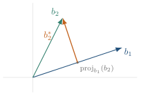
This formula generalizes directly to an algorithm: process the basis vectors one at a time, and for each one subtract off its projection onto every previously orthogonalized direction.

8.9Sage experiment: Gram–Schmidt#

B = matrix(QQ, [[2, 1], [1, 3]])
B.gram_schmidt()

The output is a set of orthogonal vectors derived from the original basis. These are not necessarily lattice vectors themselves, but they are extremely useful for analysis.

8.9.1Verification#

u = vector(QQ, [2, 1])
v = vector(QQ, [-1, 2])
u.dot_product(v)

The dot product should be \(0\), showing that the two vectors are orthogonal.

8.10Why Gram–Schmidt does not change the lattice#

This is a subtle but important point. The Gram–Schmidt vectors are not usually integer vectors, and they may not lie in the lattice at all. They are analysis tools, not new lattice generators. Their role is to reveal the geometry of the lattice basis rather than to replace it.

8.11Gram–Schmidt lengths#

The lengths of the Gram–Schmidt vectors,

\[\|b_i^*\|,\]

are a key measure of basis quality. If the lengths decrease smoothly and remain reasonably balanced, then the basis is good. If one vector becomes extremely short and another extremely long, the basis is poor.

8.12Orthogonality defect#

A useful measure of quality is the orthogonality defect. One version is

\[\mathrm{OD}(B)=\frac{\prod_i \|b_i\|}{\det(B)}.\]

If the basis vectors are perfectly orthogonal, the defect is \(1\). The larger the defect, the worse the basis.

8.13Hadamard ratio#

Another standard quantity is the Hadamard ratio:

\[\mathrm{HR}(B)=\left(\frac{\det(B)}{\prod_i \|b_i\|}\right)^{1/n}.\]

It ranges between \(0\) and \(1\), and values closer to \(1\) indicate better basis quality.

8.14Why LLL uses Gram–Schmidt repeatedly#

The LLL algorithm [2] is built around the idea that a basis can be improved by repeatedly examining the Gram–Schmidt information. If the current basis is not sufficiently reduced, LLL swaps vectors, rescales, and recomputes the orthogonalized directions until the basis quality is acceptable.

This is why Gram–Schmidt is not just a side concept: it is the engine behind one of the most important lattice reduction algorithms. The algorithm alternates between two operations: size reduction, which uses the \(\mu_{i,j}\) coefficients to make each \(b_i\) as close as possible to the span of the earlier vectors without changing the lattice, and the Lovász condition, a test on consecutive Gram–Schmidt lengths that decides whether two neighboring vectors should be swapped.

Every swap strictly decreases a potential function built from the Gram–Schmidt lengths, so the loop terminates; in practice it converges in a small number of passes even in the hundreds of dimensions used by lattice-based cryptosystems. The output is not the shortest possible basis, but it is provably short enough – each \(\|b_i\|\) is bounded in terms of the true shortest vector – to make LLL the workhorse preprocessing step before any serious lattice attack.

8.15Connection to LWE#

This chapter also helps explain why lattice problems are hard. In LWE, the secret and error are hidden in a high-dimensional structure. If an attacker could obtain a good basis for the associated lattice, many related tasks would become much easier. The security of lattice-based cryptography rests on the assumption that such a basis is not easily obtainable.

8.16Experiments#

8.16.1Experiment 1: orthogonality#

u = vector(QQ, [1, 0])
v = vector(QQ, [0, 1])
u.dot_product(v)

8.16.2Experiment 2: compare two vector pairs#

u = vector(QQ, [100, 99])
v = vector(QQ, [101, 100])
u.dot_product(v)

Compare the result with the previous experiment.

8.16.3Experiment 3: Gram–Schmidt in Sage#

B = random_matrix(QQ, 3)
B.gram_schmidt()

8.16.4Experiment 4: orthogonality defect#

Generate several random bases and compare their orthogonality defect values.

8.17Summary#

This chapter introduced the geometric notion of basis quality. Gram–Schmidt orthogonalization is not a new lattice construction; it is a way of analyzing a basis by separating old directions from genuinely new ones. A good basis is short and nearly orthogonal, while a bad basis is long and nearly parallel. These ideas are the direct precursor to LLL and other reduction algorithms.

The next chapter, Shortest Vector Problem (SVP), will connect these geometric ideas to a concrete hard problem. From there, the book turns to noise distributions and the learning with errors problem, explaining why lattice problems are so closely tied to the security of modern post-quantum cryptography.

References