PDF Run this chapter's code LaTeX source Comments
Chapter 15Centered Binomial Distribution (CBD) – Why Kyber does not use Gaussian
15.1A very important chapter#
This chapter is one of the most underestimated chapters in the whole Kyber story. Many introductions to Kyber say only that CBD is just counting a few bits. That is true, but it misses the deeper point. The real story is that CBD is not merely a convenient trick. It is a design choice that connects lattice cryptography, implementation security, hardware efficiency, and standardization history.
The central question is simple:
Why did NIST ultimately choose CBD instead of the more traditional discrete Gaussian for ML-KEM?
By the end of this chapter, you should be able to explain what CBD is, why it is close to a Gaussian, what the parameter \(\eta\) means, how FIPS 203 Algorithm 2 works, and why CBD is so attractive for constant-time implementations.
15.2Recall the LWE viewpoint#
In LWE, the core object is noise:
\[\mathbf{b}=A\mathbf{s}+\mathbf{e}.\]
The security does not come from the matrix \(A\) alone, nor from the secret \(\mathbf{s}\) alone. The crucial ingredient is the noise vector \(\mathbf{e}\).
In other words, the whole cryptographic hardness is tied to the fact that the error term hides the secret in a way that is hard to recover. A good sampling distribution for that error is therefore essential.
15.3The main problem with Gaussian sampling#
In the original theoretical LWE constructions, one often uses a discrete Gaussian distribution. A sample is drawn from a distribution of the form
\[\Pr[X=x] \propto e^{-x^2/(2\sigma^2)}.\]
This is mathematically elegant, but from an engineering point of view it is painful.
The practical issue is that Gaussian sampling usually requires expensive operations:
computing exponentials;
comparing floating-point values;
rejection sampling;
repeated loops until a sample is accepted.
This is slow, especially in software. It is also more difficult to make constant-time.
A very important side effect appears in implementation security. If a sampler uses rejection loops and branching, the running time may depend on the sampled value. This opens the door to timing attacks, where an attacker observes the timing pattern and tries to infer information about the hidden noise.
For a cryptosystem designed for real-world deployment, this is a serious drawback.
15.4Kyber’s key idea#
Kyber does not try to use the idealized Gaussian in the naive way. Instead, it asks a more practical question:
Can we construct a distribution that looks like a Gaussian, but is made only from small integers, bits, and simple arithmetic?
The answer is yes, and that answer is CBD.
CBD is simple, integer-only, and very friendly to constant-time implementation. It is much easier to deploy on hardware and software than a Gaussian sampler.
15.5The simplest example#
Let us begin with the smallest nontrivial case: \(\eta=2\).
Suppose we sample four random bits:
1010Split them into two groups of two bits:
10 10Count the number of ones in each half:
first half: \(10 \Rightarrow 1\)
second half: \(10 \Rightarrow 1\)
Now subtract:
\[1-1 = 0.\]
This gives one sampled value.
Now consider another example:
1110Then
first half: \(11 \Rightarrow 2\)
second half: \(10 \Rightarrow 1\)
and therefore
\[2-1 = 1.\]
Finally, take
0011Then
first half: \(00 \Rightarrow 0\)
second half: \(11 \Rightarrow 2\)
so
\[0-2 = -2.\]
Thus the possible values are
\[-2,-1,0,1,2.\]
15.6Why it is called centered#
The key word in the name is centered.
In a large number of samples, the positive outcomes and negative outcomes balance out. For example, values such as \(-2\) and \(2\) are rare, while \(0\) is the most common. The distribution is centered around zero.
In fact, the mean is exactly zero because the two halves contribute equally in expectation.
So the distribution is centered around zero, and that is exactly what we need for LWE noise.
15.7Why it becomes increasingly Gaussian-like#
The beautiful mathematical reason is that each bit behaves like a Bernoulli random variable:
\[B_i \in \{0,1\}, \qquad \Pr(B_i=0)=\Pr(B_i=1)=\frac{1}{2}.\]
Now consider the sum of many such Bernoulli variables. By the central limit theorem, the sum of many independent Bernoulli variables becomes approximately Gaussian.
CBD is built from exactly this phenomenon. It is not a crude heuristic. It is a discrete distribution that is mathematically close to a Gaussian because it is formed from the difference of two binomial counts.
So the real logic is:
CBD is not merely trying to look like Gaussian. It is a discrete construction whose shape naturally approaches a Gaussian-like bell curve.
15.8What does \(\eta\) mean?#
The parameter \(\eta\) controls the size of the sample.
If \(\eta=2\), we use two bits in the first half and two bits in the second half.
If \(\eta=3\), we use three bits in each half.
In general, we define
\[X = \sum_{i=1}^{\eta} B_i - \sum_{i=\eta+1}^{2\eta} B_i,\]
where each \(B_i\) is a random bit.
The resulting range is
\[-\eta, -\eta+1, \dots, \eta.\]
So larger \(\eta\) means larger noise magnitude and therefore a broader distribution.
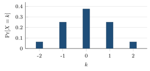
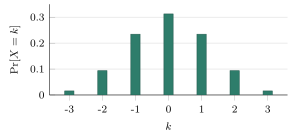
15.9Real ML-KEM parameter choices#
In the actual ML-KEM parameter sets, the values of \(\eta_1\) and \(\eta_2\) are not arbitrary. They are chosen according to security and decryption failure requirements.
| Parameter set | \(\eta_1\) | \(\eta_2\) |
|---|---|---|
| ML-KEM-512 | 3 | 2 |
| ML-KEM-768 | 2 | 2 |
| ML-KEM-1024 | 2 | 2 |
Here \(\eta_1\) is typically used for the secret distribution, while \(\eta_2\) is used for the encryption noise.
The important point is that these choices are not simply make it larger for more security. They are carefully tuned to balance security, correctness, and implementation efficiency.
Figure 15.1 plots the exact probability mass function for both values of \(\eta\) that actually appear above, computed directly from \(\Pr[\mathrm{CBD}(\eta)=k]=\binom{2\eta}{\eta+k}/4^{\eta}\).
15.10FIPS 203 Algorithm 2: what is happening?#
In FIPS 203, the standard describes a sampling procedure that is essentially the CBD sampling operation.
The high-level story is very simple:
input a bit string of length \(2\eta\);
split it into two groups of length \(\eta\);
count the number of ones in each group;
subtract the two counts.
So the procedure really is:
\[\text{CBD}_{\eta}(x) = \sum_{i=0}^{\eta-1} x_i - \sum_{i=\eta}^{2\eta-1} x_i.\]
In plain words: a short input bit string is converted into a small signed integer noise sample.
That is exactly the operation that Kyber relies on in its practical implementation.
Written out precisely, with exact bit indices instead of the informal “split it into two groups” description above, this is FIPS 203’s Algorithm 2, SamplePolyCBD\(_\eta\). It does not sample one coefficient at a time from a fresh bit string; it consumes one long byte array \(B\) of \(64\eta\) bytes and slices it into \(256\) non-overlapping windows of \(2\eta\) bits each, one window per output coefficient.
Every coefficient \(f_i\) therefore reads its own private \(2\eta\)-bit slice of \(b\), starting at bit offset \(2i\eta\): the first \(\eta\) bits of the slice are counted into \(x\), the next \(\eta\) bits into \(y\), and \(f_i=x-y \bmod q\). For \(i=0\) this is exactly the “first half, second half, subtract” recipe worked out by hand above; the only new content is the explicit offset \(2i\eta\) that tells you, for every one of the \(256\) coefficients, precisely which bits of the \(64\eta\)-byte array belong to it.
15.11A simple Sage implementation#
Here is a very small version in Python.
from random import randint


def cbd(eta):
    a = 0
    b = 0

    for _ in range(eta):
        a += randint(0, 1)

    for _ in range(eta):
        b += randint(0, 1)

    return a - b
A quick test is:
for _ in range(20):
    print(cbd(2))
Typical output might be
0
1
-1
0
2
-215.12Histogram view#
To understand CBD properly, one should look at the histogram.
samples = [cbd(2) for _ in range(100000)]The distribution tends to concentrate around zero and becomes increasingly bell-shaped. This is exactly why the distribution is often described as a discrete approximation to a Gaussian.
A very simple visualization can be done with matplotlib:
from collections import Counter
import matplotlib.pyplot as plt

samples = [cbd(2) for _ in range(100000)]
cnt = Counter(samples)

plt.bar(cnt.keys(), cnt.values())
plt.show()
If we try \(\eta=2\), \(\eta=3\), and \(\eta=4\), we can see the shape become smoother and more symmetric.
15.13Why the standard does not use randint#
A subtle but important point is that the real FIPS implementations do not literally use Python’s randint(0, 1) style calls.
Instead, the standard uses a deterministic expansion from a seed through an extendable-output function such as SHAKE.
Instead, the seed is expanded deterministically: SHAKE turns it into a pseudorandom bit stream, and CBD turns those bits into the noise sample. The full pipeline is shown in Section 15.16. This design makes the noise reproducible from the seed and straightforward to integrate into a larger protocol.
15.14Why CBD is constant-time friendly#
One of the largest practical advantages of CBD is that it is easy to implement in constant time.
The operations are only:
bit counts;
additions;
subtractions.
There is no expensive rejection loop and no data-dependent if branching in the basic procedure.
This makes CBD much easier to protect against timing attacks than a Gaussian sampler with rejection steps.
15.15A small upgrade to the toy Kyber code#
If we had earlier written a toy sampler that generated small values from a simple routine, then we can now replace it with CBD-style sampling.
For example, we might write something like:
def small_poly(n):
    coeff = []
    for _ in range(n):
        coeff.append(cbd(2))
    return coeff
In this way, the toy Kyber code becomes much closer to the actual ML-KEM design.
15.16The complete noise pipeline in FIPS 203#
We can now assemble the full path that noise takes in FIPS 203, from the initial seed to a Module-LWE sample.

The noise is therefore not a mysterious floating-point object. It is a small integer, derived deterministically from a seed through a secure expansion procedure, and every step along the way is reproducible and constant-time – exactly what a standard requires.
15.17Summary#
The important lesson of this chapter is that CBD is not just a convenience trick. It is a highly practical sampling method that combines four useful properties:
It is approximately Gaussian-shaped.
It is simple to implement.
It is easy to make constant-time.
It is well suited to software and hardware deployment.
This is why CBD became the standard choice in ML-KEM rather than the more theoretically traditional Gaussian sampler.
In one sentence:
CBD delivers a noise distribution that is good enough for lattice-based security, easy to implement, and much easier to protect against side-channel attacks than Gaussian sampling.
15.18Suggested next step#
The next natural topic is the internal hash and expansion layer: why SHAKE and Keccak are so powerful, and how a short seed can generate a huge amount of pseudorandom material. That is the bridge from CBD to the actual FIPS 203 and FIPS 204 implementations.
Comments