PDF LaTeX source Comments

Chapter 10Probability and Error Distribution

10.1What is a distribution?#

Many textbooks write expressions such as \[e \leftarrow \chi,\] where the symbol \(\chi\) is a probability distribution. In plain language, this means that the value \(e\) is sampled randomly from a certain distribution.

For example, when you roll a die, the outcome is one of \[\{1,2,3,4,5,6\},\] with each value appearing with a certain probability. This is a distribution.

Formally, a distribution describes the probability of each possible outcome: \[\Pr(X=x).\]

10.2Uniform distribution#

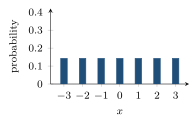
The simplest distribution is the uniform distribution. For example, suppose the value is chosen uniformly from \[\{0,1,2,3\}.\] Then each element occurs with probability \(1/4\).

In a histogram, all bars have the same height. This is the easiest notion of randomness, but it is usually not suitable for LWE noise.

If the noise were uniform over a very wide range, such as from \(-100\) to \(100\), then the resulting error would be too large for decryption to work reliably. In short, uniform noise is too wild.

10.3Gaussian distribution#

Many natural phenomena are approximately Gaussian. Examples include human height, measurement error, and random fluctuations around a mean. A Gaussian distribution is centered at zero and has a bell shape. The standard notation is \[N(0,\sigma^2),\] meaning that the mean is \(0\) and the variance is \(\sigma^2\).

The parameter \(\sigma\) controls the spread of the noise. A small \(\sigma\) means that most samples are close to zero; a large \(\sigma\) means that samples are more spread out.

10.4Why the mean is often zero#

In cryptographic noise models, the Gaussian is usually centered at zero. The reason is simple: noise should not systematically bias the system in one direction. If the error were biased, then the secret or the decrypted value might leak information.

10.5Why we cannot use continuous Gaussian directly in LWE#

The Gaussian distribution is a continuous distribution. It can produce real numbers such as \[0.1352, \quad -1.2398, \quad 2.8888.\] However, LWE is defined over a finite ring or finite field, typically modulo \(q\). The coordinates of the error must be represented as integers modulo \(q\).

Therefore, we use a discrete version of the Gaussian distribution.

10.6Discrete Gaussian#

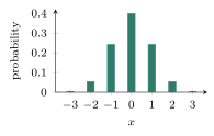
A discrete Gaussian assigns probabilities to a discrete set of integers, such as \[-3,-2,-1,0,1,2,3.\] The probabilities are larger near zero and smaller away from zero. A typical definition is \[\Pr(e=x) = \frac{e^{-x^2/(2\sigma^2)}}{Z},\] where \(Z\) is a normalization constant ensuring that the total probability is \(1\).

This kind of distribution is important because it matches the mathematical structure of lattice-based cryptography and appears in many security proofs.

10.7Why discrete Gaussian is so important#

Discrete Gaussian sampling is central in Regev-style reductions and in the theoretical analysis of lattice problems. In many proofs, the Gaussian distribution is not just convenient; it is essential. If we replace it with something else, the reduction arguments may fail.

10.8Toward CBD: the distribution Kyber ships#

Elegant as the discrete Gaussian is in theory, it is awkward in practice: sampling it well needs exponentials, floating-point comparisons, or rejection loops – all slow, and all hard to make constant-time, so that a careless sampler leaks the secret through its timing. For this engineering reason Kyber abandons the Gaussian in favour of the centered binomial distribution (CBD): a bits-only distribution, built from nothing more than sums of coin flips, whose bell shape approximates a Gaussian closely enough for security while remaining trivial to sample in constant time.

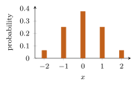
CBD is important enough – and specific enough to ML-KEM – to have a chapter of its own: Chapter 15 develops it in full, from the “count the ones in each half and subtract” recipe to the exact FIPS 203 sampling procedure and its constant-time properties. Here we only place it at the end of the progression of noise distributions.

10.9What does \(\sigma\) mean?#

In the Gaussian model, the parameter \(\sigma\) controls the magnitude of the error. If \(\sigma=0.5\), then most errors are very small. If \(\sigma=100\), then the noise is huge and the system becomes unstable. In practice, the design goal is to choose \(\sigma\) large enough to hide the secret, but small enough that decryption still succeeds with high probability.

10.10Tail bound#

Gaussian distributions are theoretically unbounded, but in practice the probability of very large errors is tiny. When cryptographers talk about the tail of a distribution, they mean the probability of values far away from the center. A short tail is useful because it means that extreme errors are rare, which helps with correctness.

10.11The noise budget#

Every scheme built on LWE and RLWE carries a small error term inside each ciphertext, and correct decryption depends on keeping that error below a fixed threshold – the noise budget. The tension is fundamental: choose the noise too small and the underlying problem becomes easy, so the scheme is insecure; choose it too large and honest decryption fails. Later chapters return to this balance when we fix concrete parameters for RLWE-based encryption and for ML-KEM, where the design drives the decryption-failure probability down to a negligible level. Managing the margin between correctness and security is one of the central practical challenges in lattice-based cryptography.

10.12Why cryptography likes Gaussian noise#

Cryptography likes Gaussian noise for three main reasons.

1. It is mathematically elegant and easy to reason about.

2. It fits naturally with lattice-based proofs and reductions.

3. It provides a strong theoretical connection to worst-case lattice hardness.

In short, noise is not there just to make things random. It is used to create a balance between correctness and security.

• If the noise is too small, the secret can be recovered more easily.

• If the noise is too large, legitimate users cannot decrypt correctly.

• The parameter choices in schemes such as \(q\), \(n\), \(\eta\), and \(\sigma\) are designed to balance these trade-offs.

10.13Summary#

The chain of ideas in this chapter runs from the simplest possible randomness to the distribution that ML-KEM actually uses: \[\text{Uniform} \;\longrightarrow\; \text{Gaussian} \;\longrightarrow\; \text{Discrete Gaussian} \;\longrightarrow\; \text{Centered Binomial Distribution (CBD)}.\] Uniform noise is easy to sample but too wild for correct decryption; the (discrete) Gaussian is the theoretically convenient choice behind most security proofs; CBD is the practical compromise that Kyber ships, built from nothing more than sums of coin flips. Figure 10.1 compares the three shapes directly: the uniform histogram is flat, while both the discrete Gaussian and CBD(\(\eta=2\)) already show the familiar bell shape, concentrated near zero.

The central idea is that noise is not merely a random artifact. It is one of the main mechanisms that makes LWE and related systems both secure and decryptable.