PDF Run this chapter's code LaTeX source Comments
Chapter 14Introduction to Kyber (ML-KEM)
14.1What is Kyber?#
Kyber – standardized by NIST as ML-KEM in FIPS 203 [1, 2] – is the post-quantum replacement for the key exchange that secures most of the internet today. It is a key-encapsulation mechanism (KEM): a protocol by which two parties establish a shared secret over a public channel, taking the role that Diffie–Hellman and RSA key transport played in the pre-quantum world. Its hardness rests on Module-LWE (Chapter 13), the middle member of the LWE family developed in the previous chapters.
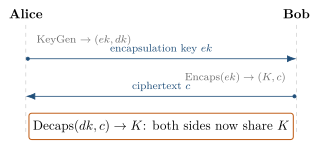
A KEM is defined by three algorithms:
KeyGen \(\to (ek, dk)\) – produce a public encapsulation key \(ek\) and a secret decapsulation key \(dk\);
Encaps\((ek)\,\to (K, c)\) – generate a fresh shared secret \(K\) together with a ciphertext \(c\) that carries it;
Decaps\((dk, c)\,\to K\) – recover the same shared secret \(K\) from the ciphertext.
Crucially, a KEM transports a random secret rather than a chosen message. That single design choice is what later lets the Fujisaki–Okamoto transform upgrade Kyber to security against active, chosen-ciphertext attackers.
14.2The pieces, and where this book builds them#
Kyber is not a new primitive. It is a careful assembly of parts developed across this book, and this chapter is where they first come together – in miniature. Some pieces are already in hand (the Module-LWE relation, the ring, the NTT); the toy below still shortcuts the others, which the cited chapters supply in full.
| Ingredient | Role in Kyber | Built in |
|---|---|---|
| Module-LWE relation \(\mathbf{t}=A\mathbf{s}+\mathbf{e}\) | the underlying hard problem | Chapter 13 |
| Ring \(R_q=\mathbb{Z}_q[x]/(x^n+1)\) and NTT | fast polynomial arithmetic | Chapters 12, 6 |
| Centered binomial noise (CBD) | sampling small secrets/errors | Chapter 15 |
| Fujisaki–Okamoto transform | lifts CPA security to CCA | Chapter 16 |
| Full FIPS 203 pipeline | KeyGen / Encaps / Decaps \(+\) FO | Chapter 16 |
The three standardized parameter sets ML-KEM-512, ML-KEM-768, and ML-KEM-1024 share the same ring but use different parameter tuples: \(k=2,3,4\), \(\eta_1=3,2,2\), and \((d_u,d_v)=(10,4),(10,4),(11,5)\) respectively [1]. NIST recommends ML-KEM-768 as the default parameter set [3]; this chapter retains only a stripped-down algebraic skeleton.
14.3Building a toy Kyber#
To see the skeleton before the machinery, we now build a toy Kyber in about a hundred lines of SageMath – small enough to inspect every object by hand. Using only mathematics already covered, it generates a public key, encrypts a message, and decrypts it:

The goal is not to reproduce the full FIPS 203 standard here, but to expose its mathematical skeleton clearly. Everything runs inside SageMath in around one hundred lines so that the structure stays visible.
14.4Simplifications used in the toy version#
The real ML-KEM standard uses many sophisticated mechanisms. In the toy version, we keep only the core idea:
| Real ML-KEM | Toy Kyber |
|---|---|
| \(q=3329\) | \(q=17\) |
| \(n=256\) | \(n=8\) |
| CBD noise | \(\text{randint}(-1,1)\) |
| SHAKE/XOF | simple random generation |
| Compression | omitted |
| NTT | ordinary polynomial multiplication |
| FO transform | omitted |
| Byte encoding | omitted |
Although these simplifications are significant, the mathematical skeleton remains the same. For the module dimension we also shrink \(k\) from \(2,3,4\) down to \(k=2\), so that the objects are easy to inspect by hand.
from random import randint

q = 17
n = 8
k = 214.5Set up the ring#
We define a polynomial ring modulo \(x^8+1\). Every object we build from here on lives in this quotient ring \(R_q\).
R.<x> = PolynomialRing(GF(q))
Rq = R.quotient(x^n + 1)
a = Rq.random_element()
b = Rq.random_element()
print(a)
print(b)
print(a*b)The highest degree should remain below \(8\) because of the quotient relation.
14.6Build the module: vectors and matrices of polynomials#
For Kyber512, the module dimension is \(k=2\). That means the secret is not one polynomial but a vector of \(k\) polynomials, and the public matrix \(A\) is a \(k \times k\) matrix of polynomials.
def rand_poly():
    return Rq.random_element()

def rand_vector():
    return vector(Rq, [rand_poly() for _ in range(k)])

def rand_matrix():
    return Matrix(Rq, k, k, [rand_poly() for _ in range(k*k)])
A vector of polynomials is already the first step toward the module viewpoint, and the matrix is the object that appears inside Kyber-like constructions.
14.7Create small noise#
In real Kyber, the noise is sampled from a centered binomial distribution (CBD), which is the subject of a later chapter. For the toy version, we simply use small coefficients in the range \(\{-1,0,1\}\).
def small_poly():
    coeffs = []
    for _ in range(n):
        c = randint(-1, 1)
        coeffs.append(c % q)
    return Rq(coeffs)

def small_vector():
    return vector(Rq, [small_poly() for _ in range(k)])
The polynomial entries are therefore small values such as \(0\), \(1\), or \(16\) (which represents \(-1\) in \(\mathbb{F}_{17}\)). This produces small errors, which are suitable for teaching.
14.8Key generation#
The module-LWE form is very close to the standard LWE form: \[\mathbf{t}=A\mathbf{s}+\mathbf{e}.\]
We implement it as follows.
def keygen():
    A = rand_matrix()
    s = small_vector()
    e = small_vector()
    t = A * s + e
    return (A, t), s
The public key is \((A,t)\) and the secret key is \(s\).
14.9Verify the key generation process#
We can print the matrix and the resulting public value to check that the shapes and types match expectations.
(pk, sk) = keygen()
A, t = pk
print("A =")
print(A)
print("\nSecret:")
print(sk)
print("\nPublic:")
print(t)
This already looks very close to the mathematical object used in Kyber.
14.10Encoding a message bit#
For the toy version, the message is reduced to a single bit. In the real scheme, message encoding is far more subtle; here we simply map a bit to either zero or a value near the middle of the modulus range.
def encode_bit(bit):
    if bit == 0:
        return Rq(0)
    else:
        return Rq(q // 2)
This is enough to demonstrate the basic idea of hiding a bit inside the noisy linear equation.
14.11Encryption#
To encrypt a message bit, we sample a random vector \(r\) and two noise terms \(e_1,e_2\). The core equations are \[u = A^T r + e_1,\] \[v = t^T r + e_2 + m.\]
def encrypt(pk, bit):
    A, t = pk
    r = small_vector()
    e1 = small_vector()
    e2 = small_poly()
    u = A.transpose() * r + e1
    m = encode_bit(bit)
    v = t.dot_product(r) + e2 + m
    return (u, v)
The ciphertext is the pair \((u,v)\).
14.12Decryption#
The decryption step uses the secret key \(s\). The main idea is that the terms involving \(A\) and \(s\) cancel out during the algebraic expansion, leaving only a small amount of noise and the encoded message.
def decrypt(sk, cipher):
    u, v = cipher
    value = v - sk.dot_product(u)
    return value
We recover the bit by comparing circular distances to the two encoding centres, \(0\) and \(\lfloor q/2\rfloor\). In particular, the field element \(16\) represents \(-1\) and must be recognised as close to encoded zero, not as a message-one value.
def recover_bit(value):
    c = value.list()[0]
    d0 = min(c, q - c)
    d1 = min((c - q//2) % q, (q//2 - c) % q)
return 0 if d0 < d1 else 114.13Putting everything together#
A complete toy run looks like this.
# Key generation
(pk, sk) = keygen()

# Encryption
bit = 1
cipher = encrypt(pk, bit)

# Decryption
value = decrypt(sk, cipher)
print("decrypted value =", value)
print("recovered bit =", recover_bit(value))
In many runs this returns the correct bit because the noise is deliberately kept small.
14.14Why the cancellation works#
The important algebraic idea is that the public key satisfies \[\mathbf{t} = A\mathbf{s}+\mathbf{e},\] so during decryption one computes \[\mathbf{v} - \mathbf{s}^T\mathbf{u}.\] After expansion, the terms involving \(A\) and \(s\) cancel, leaving only a small error term and the message. This is the core of the Kyber-like construction.
14.15Why the scheme can fail sometimes#
This toy construction can still fail frequently because \(q=17\) is tiny and the accumulated error is not bounded as in ML-KEM. It illustrates cancellation and circular decoding, not a reliable encryption scheme. In real ML-KEM, the parameters are tuned so that the decryption failure probability is extremely small.
A simple experiment is to change the noise generator from
randint(-1, 1)to something larger, such as
randint(-2, 2)or even
randint(-5, 5)and observe that decryption errors become much more frequent. This directly illustrates the role of the noise parameter, and foreshadows why real ML-KEM controls its noise distribution so carefully.
14.16What is still missing compared with real Kyber?#
This toy implementation already captures the mathematical skeleton of ML-KEM. However, it is still far from the full standard. The following components are not yet present:
CBD sampling,
SHAKE128 / SHAKE256 and XOF-based expansion,
NTT-based polynomial multiplication,
compression and encoding,
Fujisaki–Okamoto transformation,
CCA security behavior,
constant-time implementation details.
These will be introduced gradually in later chapters.
14.17Summary#
This toy implementation captures the core idea of Kyber in a compact form. Starting from the Module-LWE relation, key generation forms \(\mathbf{t}=A\mathbf{s}+\mathbf{e}\); encryption forms \(\mathbf{u}=A^{T}\mathbf{r}+\mathbf{e}_1\) and \(v=\mathbf{t}^{T}\mathbf{r}+e_2+m\); and decryption computes \(v-\mathbf{s}^{T}\mathbf{u}\), recovering the message from the resulting small, noisy value.
The most important lesson is that Kyber is not a completely new primitive. It is a carefully engineered version of the same noisy linear structure that we have been studying throughout the book. The next chapters replace the remaining shortcuts: real CBD noise sampling (Chapter 15), and then the complete FIPS 203 implementation – key generation, encapsulation, decapsulation, and the Fujisaki–Okamoto transform – in Chapter 16.
Comments