PDF Run this chapter's code LaTeX source Comments
Chapter 13Module-LWE (MLWE)
13.1The three generations of lattice-based cryptography#
We have already seen three major stages in the development of lattice-based cryptography.
First generation: LWE. The equation is \[b = A s + e,\] where \(A\) is a random matrix. The security proof is elegant, but the representation is large and the computation is costly.
Second generation: RLWE. The matrix is replaced by a polynomial ring structure. Computation becomes much faster, but the algebraic structure becomes stronger and more specialized.
Third generation: Module-LWE. This is a compromise between the large but simple LWE construction and the compact but highly structured RLWE construction.
The historical path is therefore:

13.2What is a module?#
The word “module” is not informal jargon; it is a precise algebraic structure, and Kyber’s secrets live in one. It generalizes the vector space of Chapter 3 by letting the scalars come from a ring instead of a field.
Definition 13.1 (Module over a ring). Let \(R\) be a commutative ring with identity \(1\). A (left) \(R\)-module is an abelian group \((M,+)\) together with a scalar multiplication \(R\times M\to M\), written \((r,m)\mapsto rm\), such that for all \(r,s\in R\) and \(x,y\in M\):
\(r(x+y)=rx+ry\);
\((r+s)x=rx+sx\);
\((rs)x=r(sx)\);
\(1\,x=x\).
These are exactly the vector-space axioms with the field replaced by a ring. When \(R\) is a field, an \(R\)-module is a vector space; a module is the strictly more general object obtained by relaxing “field” to “ring.” Several properties carry over, and one convenience is lost.
Free modules and rank. The set \(R^{k}=\{(m_1,\dots,m_k):m_i\in R\}\) with componentwise operations is an \(R\)-module, the free module of rank \(k\). Like a vector space it has a basis – the standard unit vectors \(e_1,\dots,e_k\) – so every element is a unique \(R\)-combination of them. Kyber’s secret space is exactly the free module \(R_q^{k}\).
Matrices act as homomorphisms. A matrix \(A\in R^{k\times k}\) defines an \(R\)-linear map \(R^{k}\to R^{k}\), \(\mathbf{x}\mapsto A\mathbf{x}\), called an \(R\)-module homomorphism. The Module-LWE map \(\mathbf{s}\mapsto A\mathbf{s}\) is one of these.
Submodules and ideals. A submodule is the analogue of a subspace; the submodules of \(R\) regarded as a module over itself are precisely its ideals (Chapter 4) – which is why RLWE is said to rest on ideal lattices.
What is lost. Over a general ring, not every module is free and not every submodule has a basis – a real departure from vector spaces. Kyber avoids this entirely by working in the free module \(R_q^{k}\).
With the structure named precisely, the three-generation progression is a statement about which module the secret lives in: \[\underbrace{s\in\mathbb{Z}_q^{n}}_{\text{LWE}} \qquad \underbrace{s(x)\in R_q}_{\text{RLWE}} \qquad \underbrace{\mathbf{s}\in R_q^{k}}_{\text{Module-LWE}}.\] LWE uses a vector of field elements; RLWE uses a single ring element; Module-LWE uses a length-\(k\) vector over the ring \(R_q\) – a free module of rank \(k\).
13.3Kyber’s secret#
In ML-KEM (Kyber), the secret is not a single polynomial but a vector of polynomials. The security level determines the dimension of that vector.
Kyber512 uses \(k=2\).
Kyber768 uses \(k=3\).
Kyber1024 uses \(k=4\).
Thus, the security level is tied to the size of the module.
13.4Why does the matrix come back?#
At first glance, people are surprised to see matrices again in Kyber. But the matrix is not a large random matrix over integers. Instead, its entries are polynomials.
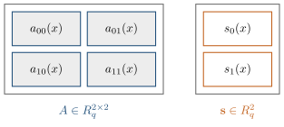
For example, for \(k=2\), we may have \[A = \begin{bmatrix} a_{11}(x) & a_{12}(x) \\ a_{21}(x) & a_{22}(x) \end{bmatrix}.\]
Each entry is a polynomial in the ring \(R_q\). The object is still a matrix, but the matrix entries are now ring elements rather than ordinary numbers.
13.5Kyber public key generation#
The public key generation is very similar to LWE in spirit. We choose a secret vector \(\mathbf{s}\), a noise vector \(\mathbf{e}\), and a polynomial matrix \(A\), and then compute \[\mathbf{t} = A\mathbf{s} + \mathbf{e}.\]
This is exactly the same governing idea as LWE, except that the scalars are now ring elements. The figure below makes the shapes of \(A\) and \(\mathbf{s}\) concrete for the smallest case \(k=2\) (indices run from \(0\) to \(k-1\), matching the Sage code below).
13.6Why is this better than plain LWE?#
We can compare the three designs.
LWE: the matrix is huge and the public key is large.
RLWE: the representation is compact, but the algebraic structure is very strong.
Module-LWE: the matrix is small and the elements are polynomials, giving a very good compromise between compactness and flexibility.
In other words, Module-LWE uses a small matrix of polynomials instead of a huge matrix of integers or a single large polynomial.
13.7Sage construction of a toy module#
We can create a very small toy example in Sage. First define the ring.
q = 17
R.<x> = PolynomialRing(GF(q))
S = R.quotient(x^8 + 1)
Now define a secret as a vector of two polynomials.
from random import choice
def small_poly():
    return S([choice([-1, 0, 1]) for _ in range(8)])

s = vector(S, [small_poly(), small_poly()])
print(s)
Create a small polynomial matrix.
A = Matrix(S, [[S.random_element(), S.random_element()],
               [S.random_element(), S.random_element()]])
print(A)
Create a noise vector.
e = vector(S, [small_poly(), small_poly()])
assert all(c in [0, 1, 16] for p in list(s) + list(e) for c in p.lift().list())
Then compute the public-like value.
t = A * s + e
print(t)
This has the algebraic shape of a Module-LWE sample. The public matrix is uniform, while the secret and error use small coefficients; it is still a toy example rather than the FIPS 203 sampler.
13.8The Module-LWE problem#
With the module structure in place, Module-LWE is the LWE distribution of Chapter 11 with the scalars promoted from \(\mathbb{Z}_q\) to the ring \(R_q\).
Definition 13.2 (Module-LWE). Fix the ring \(R_q=\mathbb{Z}_q[x]/(x^n+1)\), a module rank \(k\), and an error distribution \(\chi\) over \(R_q\) concentrated on small elements. For a secret \(\mathbf{s}\in R_q^{k}\), the Module-LWE distribution outputs \[(\mathbf{a},\,b),\qquad \mathbf{a}\leftarrow R_q^{k}\ \text{uniform},\quad e\leftarrow\chi,\quad b=\langle \mathbf{a},\mathbf{s}\rangle + e\in R_q.\] Stacking \(m\) samples as the rows of \(A\in R_q^{m\times k}\) gives the matrix form \((A,\ \mathbf{t}=A\mathbf{s}+\mathbf{e})\). Search-MLWE is to recover \(\mathbf{s}\); Decision-MLWE is to distinguish \((A,\,A\mathbf{s}+\mathbf{e})\) from a uniform pair \((A,\,\mathbf{u})\).
Two special cases bracket the definition: \(k=1\) is RLWE (a single ring element), and \(n=1\) with \(R_q=\mathbb{Z}_q\) recovers plain LWE. Module-LWE interpolates between them, and it inherits a worst-case hardness guarantee of the same flavour as LWE: solving it on average is at least as hard as standard problems on module lattices [1]. In Kyber the matrix is square (\(m=k\)), giving the compact form \[\mathbf{t} = A\mathbf{s} + \mathbf{e}, \qquad A\in R_q^{k\times k},\ \ \mathbf{s},\mathbf{e}\in R_q^{k}.\]
13.9Why Module-LWE is considered a compromise#
Many people wrongly think that Module-LWE is simply "better" because it uses more structure. That is not the correct understanding. The real point is that Module-LWE reduces the strongest algebraic structure of pure RLWE while retaining the efficiency advantages. In other words, it trades off between:
the huge size of plain LWE,
the strong structure of RLWE,
and the practical middle ground provided by MLWE.
This balance is central to Kyber’s design.
13.10Why the Kyber parameters are \(k=2,3,4\)#
The values \(k=2,3,4\) correspond to different dimensions of the module, and are exactly the three security levels of Kyber [1, 2]. In practice:
\(k=2\) gives Kyber512,
\(k=3\) gives Kyber768,
\(k=4\) gives Kyber1024.
Increasing \(k\) increases the size of the module and therefore increases the security level. The ring dimension and modulus stay fixed, but standardized ML-KEM parameter sets use different parameter tuples as well: in particular \(\eta_1\) is \(3,2,2\) and \((d_u,d_v)\) is \((10,4),(10,4),(11,5)\) for ML-KEM-512, -768, and -1024 respectively [3].
13.11A complete toy MLWE experiment#
A useful exercise is to implement a toy version of MLWE in full.
Define a ring \(R_q\).
Create a small polynomial matrix \(A\).
Create a polynomial vector \(\mathbf{s}\).
Create a noise vector \(\mathbf{e}\).
Compute \(\mathbf{t}=A\mathbf{s}+\mathbf{e}\).
Print the result and inspect its structure.
This gives a practical understanding of why Kyber can be seen as a structured generalization of LWE. Written as pseudocode, using the same names \(A\), \(\mathbf{s}\), \(\mathbf{e}\), \(\mathbf{t}\) as the Sage code above, the same six steps are Algorithm 11.
Real ML-KEM has this algorithmic shape with \(n=256\) and \(k=2,3,4\), but the standardized parameter sets differ in more than \(k\); their sampling and compression parameters are specified in FIPS 203.
13.12Summary#
The key lesson is that Module-LWE is not merely "LWE with more polynomials". It is the middle ground between the two extremes:
| Scheme | Secret object | Main idea |
|---|---|---|
| LWE | vector over \(\mathbb{Z}_q\) | simple and general, but large |
| RLWE | single polynomial over \(R_q\) | compact and fast, but highly structured |
| Module-LWE | vector of polynomials over \(R_q\) | balanced compromise, used by Kyber |
The important insight is that Kyber is not simply RLWE with a different name. It is the module version of the same noisy linear structure, arranged in a way that gives practical efficiency while preserving strong security assumptions.
Comments