PDF Run this chapter's code LaTeX source Comments

Chapter 7Lattices

7.1Why this chapter matters#

This chapter is one of the most important in the whole course. If the previous chapters introduced vectors, matrices, and polynomial rings, then this chapter explains the geometric object that makes post-quantum cryptography possible: the lattice. Lattices are the core structure behind LWE, RLWE, Kyber, Dilithium, and many other modern constructions.

7.2Learning goals#

After reading this chapter, you should be able to:

• explain what a lattice is;

• distinguish a lattice from a vector space;

• understand why a lattice can have many different bases;

• understand the difference between good and bad bases;

• appreciate why problems such as SVP and CVP are difficult;

• see the connection between lattice problems and LWE.

7.3Starting from two dimensions#

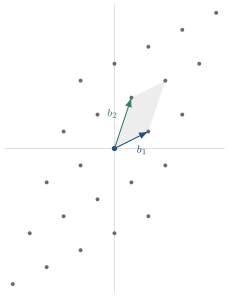
Instead of jumping immediately to high-dimensional theory, begin with a simple two-dimensional example. Let

\[b_1 = \begin{pmatrix}2\\1\end{pmatrix}, \qquad b_2 = \begin{pmatrix}1\\3\end{pmatrix}.\]

Now allow only integer coefficients:

\[v = x b_1 + y b_2, \qquad x,y \in \mathbb{Z}.\]

If we take many such combinations, the resulting points form an infinite regular pattern of discrete points in the plane. This set is called a lattice.

7.3.1Sage experiment: generate a two-dimensional lattice#

b1 = vector(ZZ, [2, 1])
b2 = vector(ZZ, [1, 3])
points = []
for i in range(-5, 6):
    for j in range(-5, 6):
        points.append(i * b1 + j * b2)
points[:10]

The output is a list of lattice points. The important observation is that they are arranged in a very regular, discrete pattern.

7.4Formal definition#

Formally, if \(b_1, \ldots, b_n\) are linearly independent vectors, then the set

\[L(B) = \left\{ \sum_{i=1}^{n} z_i b_i \;:\; z_i \in \mathbb{Z} \right\}\]

is called the lattice generated by the basis \(B = \{b_1, \ldots, b_n\}\).

The key difference from a vector space is that the coefficients are restricted to integers rather than arbitrary real numbers.

This definition is directly executable: enumerating a lattice inside a bounded region is exactly a bounded search over integer coefficient vectors.

This is precisely what the Sage experiment above does for \(n=2\) and \(N=5\): two nested loops over integer coefficients, collecting every resulting point. The regular grid in Figure 7.1 is the output of this algorithm.

7.5Why a lattice is not a vector space#

A vector space allows arbitrary real or complex coefficients. For example,

\[0.13 b_1 + 2.78 b_2\]

is a perfectly valid element of the vector space spanned by \(b_1\) and \(b_2\). But in a lattice, the coefficients must be integers. That is why the lattice is a discrete structure rather than a continuous one.

This distinction is crucial. Cryptography needs discrete problems because continuous problems are often easy to solve.

7.6Vector space versus lattice#

A vector space is continuous and dense. A lattice is discrete and sparse. In other words:

• vector space: all linear combinations with real coefficients;

• lattice: only integer linear combinations.

This difference is exactly why lattice problems are hard and useful for cryptography.

7.7A lattice can have many bases#

The most important conceptual point is that a lattice can be described by many different bases. For example, the basis

\[\left\{(1,0), (0,1)\right\}\]

and the basis

\[\left\{(2,1), (1,1)\right\}\]

can generate the same lattice.

This is similar to how a city can be described using different coordinate systems. The city does not change, only the coordinate description does.

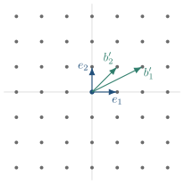
\(e_1=(1,0),\ e_2=(0,1) \qquad b_1'=(2,1),\ b_2'=(1,1)\)

7.7.1Sage experiment: two different bases#

B1 = matrix(ZZ, [[1, 0], [0, 1]])
B2 = matrix(ZZ, [[2, 1], [1, 1]])

Later, we will verify that these generate the same lattice.

7.8Good bases and bad bases#

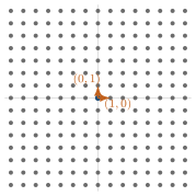
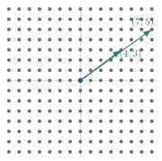
Now we arrive at the central idea behind lattice reduction. Some bases are good and some are bad.

A bad basis is made of vectors that are nearly parallel and long. Such a basis makes it hard to find nearby lattice points.

A good basis consists of relatively short and nearly orthogonal vectors, which makes the lattice easier to navigate.

This is the reason that algorithms such as LLL and BKZ exist: they try to transform a bad basis into a better one.

7.9Fundamental parallelepiped#

Given a basis, we can form the fundamental parallelepiped, the basic cell of the lattice. Its volume is related to the determinant of the basis matrix.

For a two-dimensional lattice, the area of this cell is given by the absolute value of the determinant.

7.9.1Sage experiment: determinant#

B = matrix(ZZ, [[2, 1], [1, 3]])
B.det()

The determinant is a measure of how dense the lattice is. A larger determinant usually means a sparser lattice, while a smaller determinant means a denser one.

7.10Lattice dimension#

In two dimensions, a lattice is easy to visualize. In cryptography, however, the dimension is much larger. Kyber, Dilithium, and other lattice-based systems may work in dimensions of hundreds or even thousands. In these high-dimensional spaces, geometry becomes much harder to picture, but much of the same intuition still applies.

7.11Why lattice problems become hard#

In low dimensions, one can often solve lattice problems by hand or by simple geometric arguments. In higher dimensions, however, the search for short vectors or nearby vectors becomes extremely difficult. This explosion in complexity is the foundation of lattice-based security.

7.12Sage experiment: shortest vector#

Sage provides built-in lattice tools. A lattice object can be created directly from an integer matrix as follows:

from sage.modules.free_module_integer import IntegerLattice

B = matrix(ZZ, [[2, 1], [1, 3]])
L = IntegerLattice(B)
L

Once the lattice is defined, the shortest vector can be computed with a single command:

L.shortest_vector()

This is the basic object behind the shortest vector problem (SVP), one of the central hardness assumptions in lattice-based cryptography.

7.13Experiments#

The lattices underlying ML-KEM (FIPS 203 [1]) and ML-DSA (FIPS 204 [2]) live in dimensions of several hundred, where their geometry cannot be visualized. The following experiments isolate, in two dimensions where every object can be drawn and checked by hand, the four phenomena on which those standards ultimately depend: the discreteness of the point set, the basis-invariance of the determinant, the gap between good and bad bases, and the intractability of the shortest vector. Each recurs unchanged in principle at cryptographic scale.

7.13.1Experiment 1: enumerating the lattice#

Generate a finite window of the lattice \(\Lambda(\mathbf{b}_1,\mathbf{b}_2)\) and confirm that it is a discrete grid of points, not a continuous span.

b1 = vector(ZZ, [2, 1])
b2 = vector(ZZ, [1, 3])
pts = [i * b1 + j * b2 for i in range(-4, 5) for j in range(-4, 5)]
pts

Plotting pts reveals the characteristic regular grid. This is the same object that, in dimension \(256\) and over \(\mathbb{Z}_q\) rather than \(\mathbb{Z}\), becomes the module lattice at the core of ML-KEM.

7.13.2Experiment 2: the determinant is a basis invariant#

Compute the lattice determinant \(\det\Lambda = |\det B|\) for several bases of the same lattice, each obtained by left-multiplying \(B\) by a unimodular matrix \(U \in \mathrm{GL}_n(\mathbb{Z})\) (an integer matrix with \(\det U = \pm 1\)).

B = matrix(ZZ, [[2, 1], [1, 3]])
U = matrix(ZZ, [[1, 0], [1, 1]])          # unimodular: det U = 1
print(abs(B.det()), abs((U * B).det()))   # identical

The determinant – the covolume of the fundamental parallelepiped, and hence the inverse density of the lattice – is unchanged, while the basis vectors themselves change completely. This invariance under \(\mathrm{GL}_n(\mathbb{Z})\) is precisely what allows a scheme to publish one basis of a lattice while holding another in secret.

7.13.3Experiment 3: good bases versus bad bases#

A single lattice admits both near-orthogonal (“good”) and highly skewed (“bad”) bases. Contrast the two, and quantify the skew through the orthogonality defect \(\prod_i \lVert \mathbf{b}_i\rVert / \det\Lambda\).

good = matrix(ZZ, [[1, 0], [0, 1]])       # orthonormal basis of Z^2
bad  = matrix(ZZ, [[1, 7], [0, 1]])       # a sheared basis of the same Z^2

This gap is the heart of trapdoor lattice cryptography. In the NTRU-based FN-DSA and, in spirit, throughout ML-DSA (FIPS 204 [2]), the secret key behaves as a good basis and the public key as a bad one; forging a signature without the good basis reduces to a hard lattice problem. Chapter 8 makes the good/bad distinction quantitative and shows how far a bad basis can be reduced toward a good one.

7.13.4Experiment 4: the shortest vector is a lattice invariant#

Compute the shortest nonzero vector for several distinct bases of the same lattice and confirm that its length is a property of the lattice, not of the chosen basis.

from sage.modules.free_module_integer import IntegerLattice
B1 = matrix(ZZ, [[2, 1], [1, 3]])
B2 = matrix(ZZ, [[3, 4], [4, 7]])          # = U*B1, U unimodular: same lattice
for B in [B1, B2]:
    print(IntegerLattice(B).shortest_vector())   # identical length

In two dimensions shortest_vector answers instantly. In the dimensions of FIPS 203 and 204 no known algorithm does so in feasible time, and that asymptotic intractability – formalized as the shortest vector problem (SVP), together with its approximate and decisional variants – is the security foundation on which both standards rest.

7.14Summary#

The main lessons of this chapter are threefold:

1. A lattice is not a vector space; it is a discrete structure formed by integer linear combinations.

2. A lattice can have many different bases, and the choice of basis strongly affects how easy or hard the lattice is to work with.

3. The hardness of lattice problems, especially SVP and CVP, is the foundation of many post-quantum cryptosystems.

The next chapter, Gram–Schmidt Orthogonalization and the LLL Algorithm, will introduce the first major algorithmic tool for turning a bad basis into a good one.

References