PDF LaTeX source Comments

Chapter 22Classic McEliece

22.1Learning objectives#

So far the book has drawn on two hard-problem families: lattices (ML-KEM, ML-DSA, FN-DSA) and hash functions (SLH-DSA). This part opens a third, entirely independent foundation. Code-based cryptography does not ask you to find short vectors in a lattice; it asks you to decode a random-looking linear code. It is the oldest post-quantum family of all – Robert McEliece proposed his scheme in 1978, the same year RSA appeared [1] – and after more than forty years of attack it stands essentially unbroken. That track record is precisely why it is prized: where the lattice standards trade a little conservatism for small keys and speed, Classic McEliece makes the opposite bet.

After finishing this chapter, you should be able to:

1. state the basic objects of a binary linear code – generator matrix, parity-check matrix, Hamming weight and distance, and the syndrome of an error;

2. explain the syndrome decoding problem and why its NP-hardness (with no known quantum shortcut beyond Grover) is the security foundation of the scheme;

3. describe the trapdoor: a secret code that can be decoded efficiently, disguised as a code that cannot;

4. follow the KeyGen, Encapsulate, and Decapsulate algorithms and see exactly where the secret decoder is used;

5. explain the trade-off Classic McEliece makes – very large public keys in exchange for tiny ciphertexts and a long, conservative security record.

Why this chapter matters.#

Code-based cryptography is one of the three problem families named in the Quantum Threat chapter (Chapter 1), alongside lattices and hashes. Each is a different bet against an uncertain quantum future, and the value of holding more than one bet is that they fail independently: a breakthrough against lattices would say nothing about codes. Classic McEliece is the flagship of the code-based hedge. Understanding it also completes the picture of what “post-quantum” means – not one idea, but several unrelated hard problems, any one of which could carry public-key cryptography through the quantum era.

22.2A crash course in linear codes#

The reader has met lattices and polynomial rings but not, so far, coding theory. This section builds the handful of objects the scheme needs. Everything lives over the binary field \(\mathbb{F}_2 = \{0,1\}\), where addition is XOR.

Codes as subspaces.#

A binary linear code \(C\) is simply a linear subspace of \(\mathbb{F}_2^n\). If that subspace has dimension \(k\), we call \(C\) an \([n,k]\) code: it contains \(2^k\) codewords, each an \(n\)-bit string. The idea is redundancy. We take a \(k\)-bit message and spread it across \(n > k\) bits, so that if a few of those bits are flipped in transit we can still recover the original.

The generator matrix.#

Because \(C\) is a \(k\)-dimensional subspace, it has a basis of \(k\) codewords. Stacking that basis as the rows of a \(k \times n\) matrix \(G\) gives the generator matrix. Encoding a message \(m \in \mathbb{F}_2^k\) is then a single matrix product: \[c = m\,G \in \mathbb{F}_2^n .\] As \(m\) ranges over all \(2^k\) messages, \(mG\) ranges over all codewords. The generator matrix is the code, written down.

The parity-check matrix.#

The same subspace can be described from the outside, by the linear constraints its codewords satisfy. The parity-check matrix \(H\) is an \((n-k) \times n\) matrix whose null space is exactly \(C\): \[H\,c^\top = 0 \quad\text{for every codeword } c \in C .\] So \(G\) tells you how to build codewords and \(H\) tells you how to recognize them. The two are linked by \(G H^\top = 0\).

Weight, distance, and error correction.#

The Hamming weight \(\mathrm{wt}(x)\) of a vector is the number of nonzero coordinates, and the Hamming distance between two vectors is the weight of their difference, \(d(x,y) = \mathrm{wt}(x-y)\). The minimum distance \(d\) of a code is the smallest distance between two distinct codewords. A code with minimum distance \(d\) can correct up to \[t = \left\lfloor \tfrac{d-1}{2} \right\rfloor\] bit errors: if a codeword is corrupted in at most \(t\) positions, it is still closer to the original codeword than to any other, so the original can in principle be recovered.

The syndrome.#

Suppose a codeword \(c\) is sent and arrives as \(y = c + e\), where \(e\) is an unknown error vector. Multiplying the received word by the parity-check matrix gives \[s = H\,y^\top = H\,c^\top + H\,e^\top = H\,e^\top ,\] because \(Hc^\top = 0\). The result \(s \in \mathbb{F}_2^{\,n-k}\) is the syndrome. Two things are worth pausing on. First, the syndrome depends only on the error, not on which codeword was sent. Second, decoding – recovering \(e\) (and hence \(c\)) – is exactly the task of finding a low-weight \(e\) that produces the observed syndrome. This single observation is the hinge of the entire chapter.

22.3The hard problem: syndrome decoding#

For a code with helpful structure, decoding is easy – that is the whole point of designing codes. But strip the structure away and the picture inverts.

Syndrome Decoding. Given a random parity-check matrix \(H \in \mathbb{F}_2^{(n-k)\times n}\), a target syndrome \(s \in \mathbb{F}_2^{\,n-k}\), and a weight \(t\), find an error vector \(e\) with \(\mathrm{wt}(e) \le t\) and \(H\,e^\top = s\).

For a code with no exploitable structure, this is genuinely hard. It was proved NP-complete by Berlekamp, McEliece, and van Tilborg in 1978 [2] – the same year the encryption scheme was proposed. Intuitively, the linear system \(He^\top = s\) has many solutions, but almost all of them have large weight; the constraint \(\mathrm{wt}(e) \le t\) picks out an exponentially rare needle, and there is no linear-algebra shortcut to it.

The best known attacks are the family of information-set decoding (ISD) algorithms, refined steadily since the 1960s. They run in time exponential in the code parameters, and decades of optimization have improved only the constant in the exponent, never removed it. Crucially, quantum computers do not change this picture qualitatively: the strongest quantum variants apply Grover-style search inside ISD and gain at most a square-root speedup, exactly the mild erosion the Quantum Threat chapter described for all the post-quantum families. There is no Shor-like collapse. Doubling the parameters restores the lost margin, just as it does for a symmetric cipher.

This is the security foundation. If we can present an attacker with what looks like a random parity-check matrix and a syndrome, and the secret is a low-weight error, then breaking the scheme means solving syndrome decoding.

22.4The trapdoor: a decodable code in disguise#

The problem, of course, is that the honest parties also see only the public matrix. If it were truly random, nobody could decode, and the scheme would be useless. The resolution is the central trick of trapdoor cryptography: start from a code that does have an efficient decoder, then disguise it so thoroughly that from the outside it is indistinguishable from a random code.

The secret code.#

Classic McEliece builds its secret from a binary Goppa code. The full construction, parameters, and decoding of these codes are developed in Appendix A; here the two properties we rely on are simple to state:

• it is an \([n,k]\) linear code, with a generator matrix \(G\), chosen so that it can correct \(t\) errors;

• it comes with an efficient \(t\)-error decoding algorithm \(\mathcal{D}_g\) (Patterson’s algorithm), which takes any word within distance \(t\) of a codeword and returns the codeword and the error.

Goppa codes are the workhorse here for a specific reason: after four decades of scrutiny, a scrambled Goppa code still cannot be told apart from a random linear code by any known efficient test. Other code families that looked equally promising (for instance, certain algebraic codes) were later shown to leak their structure and were broken. Goppa codes have held.

The disguise.#

Two secret ingredients hide the structure:

• a random invertible scrambler matrix \(S\) of size \(k \times k\) over \(\mathbb{F}_2\), which mixes the rows of \(G\) (it changes the basis, not the code);

• a random \(n \times n\) permutation matrix \(P\), which shuffles the coordinates.

The public key is the transformed generator matrix \[G' = S\,G\,P .\] Scrambling by \(S\) and permuting by \(P\) both preserve the fact that this is some \([n,k]\) code, but they destroy every visible trace of the Goppa structure that made \(G\) decodable. To anyone without \(S\), \(P\), and \(\mathcal{D}_g\), the matrix \(G'\) is just a random-looking code with no known efficient decoder.

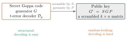
The asymmetry in the caption is the whole scheme in one sentence. Encryption adds a weight-\(t\) error to a public codeword; this is easy for anyone. Decryption removes that error; this is easy only for the trapdoor holder and, for everyone else, is syndrome decoding.

22.5The scheme#

We present two views of the same idea. The original 1978 form encrypts a message directly and is the clearest illustration of the trapdoor. The modern form – the one the NIST “Classic McEliece” submission [3] actually specifies – is a key-encapsulation mechanism (KEM) built on the dual, parity-check description of the code. Both rely on the same secret decoder.

22.5.1The original 1978 encryption#

Key generation produces the disguise of the previous section: a secret Goppa code with decoder \(\mathcal{D}_g\), a scrambler \(S\), a permutation \(P\), and the public generator \(G' = SGP\).

To encrypt a message \(m \in \mathbb{F}_2^k\), the sender encodes it against the public matrix and deliberately adds a fresh random error \(e\) of weight exactly \(t\): \[c = m\,G' + e , \qquad \mathrm{wt}(e) = t .\] The ciphertext \(c\) is a codeword of the public code, knocked off the code in \(t\) positions. To an eavesdropper, recovering \(m\) means removing \(e\) – syndrome decoding of a random-looking code.

To decrypt, the receiver peels the disguise off one layer at a time, and this is where the secret is spent. The key algebraic fact is that a permutation only reshuffles the error’s positions, so it never changes its weight.

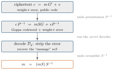
Written out, decryption is: compute \(cP^{-1} = mSG + eP^{-1}\), which is a Goppa codeword \(mSG\) corrupted in exactly \(t\) positions; run \(\mathcal{D}_g\) to strip the error and read off \(mS\); then multiply by \(S^{-1}\) to get \(m\). Without the secret decoder, the second step is impossible, and that is the whole security of the scheme.

22.5.2The modern KEM: sending a syndrome#

The NIST submission uses the Niederreiter presentation [4], which is the dual of the picture above. Instead of a scrambled generator matrix it publishes a scrambled parity-check matrix, and instead of encrypting a chosen message it encapsulates a random key. This form has smaller ciphertexts and is what you should think of as “Classic McEliece” today.

The public key is now a disguised parity-check matrix \[H' = S\,H\,P ,\] where \(H\) is the parity-check matrix of the secret Goppa code, \(S\) is an invertible \((n-k)\times(n-k)\) scrambler, and \(P\) is again a coordinate permutation. (In the actual specification \(H'\) is reduced to systematic form \([\,I \mid T\,]\), so only the sub-block \(T\) needs to be stored; the scrambler \(S\) is exactly the row reduction that achieves this. We keep \(S\) explicit here for clarity.)

The idea of encapsulation is that the secret is a low-weight error vector, and the ciphertext is its syndrome. Because the syndrome of a weight-\(t\) error under a random-looking \(H'\) is a hard thing to invert, the ciphertext hides the error from everyone but the trapdoor holder. The shared key is then derived by hashing that error.

Encapsulation never touches the secret. It just samples a random error of the prescribed weight and reports its syndrome.

Decapsulation is where the trapdoor is spent. The receiver undoes the scrambler, hands the result to the secret Goppa decoder to recover a permuted error, then undoes the permutation and re-hashes – arriving at the same key the sender computed.

The correctness is the mirror of Figure 22.2: multiplying by \(S^{-1}\) turns the public ciphertext \(c = SHP\,e^\top\) into \(H(Pe^\top)\), a genuine syndrome of the Goppa code for a permuted-but-same-weight error; the decoder \(\mathcal{D}_g\) recovers that error because its weight is exactly \(t\); undoing \(P\) restores the original \(e\); and hashing \(e\) reproduces the sender’s key. An attacker who sees only \(H'\) and \(c\) is left with syndrome decoding.

A note on real-world hardening.#

The teaching form above sets \(K = \mathrm{Hash}(e)\). To achieve security against active (chosen-ciphertext) attackers, the actual specification hashes the ciphertext into the key as well and uses implicit rejection: if decoding fails or the recovered error has the wrong weight, decapsulation does not abort but returns a pseudorandom key derived from a secret stored in the key. This hides from the attacker whether decoding succeeded, closing a class of reaction attacks. The essential structure – error in, syndrome out, decode with the trapdoor – is exactly as shown.

22.6Trade-offs and status#

Classic McEliece makes an unusual and deliberate trade. Its public key is enormous – a dense matrix of hundreds of kilobytes, up to about a megabyte at the highest security level – because the public key essentially is a random-looking code, and there is no seed to compress it down to (contrast the lattice standards, where the public matrix regenerates from a 32-byte seed). But everything else is small and fast: the ciphertext is merely a syndrome, well under a few hundred bytes, and encapsulation and decapsulation are quick. Where a lattice KEM balances all its sizes, Classic McEliece pushes the entire cost into a one-time, static public key that can be generated once and reused for a long time.

Status.#

Classic McEliece competed in the NIST post-quantum project as a key-encapsulation candidate and advanced into the fourth round dedicated to additional KEMs. It is not a published NIST FIPS, and NIST IR 8545 selected HQC rather than Classic McEliece for the additional-KEM standardization path. Classic McEliece nevertheless has the longest public cryptanalytic record of any scheme in this book, and that record is why it is worth studying.

That record is currently moving.#

Since 2023 a line of structural attacks has been closing on the parameter sets themselves. None of them decrypts anything, and none recovers a key at standardized parameters; what they attack is the indistinguishability of the public key from a random matrix. The most recent, of Ghoshal, Ishai, Jain and Sun [5], is quasipolynomial-time, applies to every parameter set NIST considered, and — on the smallest set — costs fewer operations than generic decoding does. Appendix A works through how it does that and what it leaves standing, because the mechanism is instructive well beyond this one scheme.

The honest summary is a two-part one, and the two parts are easy to conflate:

• the minimal assumption — recovering a message means decoding, which is hard — is intact, and no attack has come near it;

• the conservative assumption — the public key is indistinguishable from random, which is the one usually invoked when McEliece is called the safe choice — no longer holds at any standardized parameter set.

A reader deciding whether to deploy this should weigh both. A reader deciding whether to study it should note that a forty-eight-year-old scheme is currently the most interesting cryptanalytic target in the field, which is not an argument against reading the chapter.

22.7Pitfalls#

Pitfall 1: thinking the large public key is a flaw to be fixed.#

The size is intrinsic. The public key is a random-looking code, and a random code has no shorter description than the matrix itself. You cannot regenerate it from a small seed the way ML-KEM regenerates its matrix \(A\), because a seed-expandable matrix would carry exploitable structure. The large key is the price of the conservative assumption, not an implementation oversight.

Pitfall 2: thinking the error weight is negotiable.#

The decoder \(\mathcal{D}_g\) corrects up to \(t\) errors and no more. Encapsulation must use weight exactly \(t\): too few and it is easier to attack, too many and honest decoding fails. The weight is a fixed scheme parameter, not a tunable knob at encryption time.

Pitfall 3: assuming any decodable code family will do.#

The security rests on the scrambled code being indistinguishable from random. Several families that offered efficient decoders (such as certain algebraic and low-density codes) were shown to leak their structure through the disguise and were broken outright. Binary Goppa codes are used because they resisted those attacks — and, as Section A.8 sets out, they now leak that structure too, at quasipolynomial rather than polynomial cost. The distinction between “leaks nothing” and “leaks expensively” is the whole of the scheme’s present margin, so it is worth keeping straight.

Pitfall 4: skipping the chosen-ciphertext hardening.#

The bare scheme in the algorithm boxes is only passively secure. Real deployments must bind the ciphertext into the key and use implicit rejection, exactly as the lattice KEMs apply a Fujisaki–Okamoto-style transform (Section 16.13). Omitting it exposes reaction attacks that learn the secret from whether decoding succeeds.

22.8Summary#

Code-based cryptography rests on a hard problem wholly separate from lattices: decoding a random linear code, formalized as syndrome decoding, which is NP-hard and enjoys no quantum shortcut beyond Grover’s mild square-root erosion. Classic McEliece turns this into a cryptosystem by the classic trapdoor manoeuvre:

• it starts from a binary Goppa code, which has an efficient \(t\)-error decoder \(\mathcal{D}_g\);

• it disguises that code with a secret scrambler \(S\) and permutation \(P\), publishing \(G' = SGP\) (or, dually, \(H' = SHP\)), which looks random;

• anyone can encapsulate – add or send a weight-\(t\) error – but only the holder of \(S\), \(P\), and \(\mathcal{D}_g\) can decapsulate, because only they can decode;

• it buys unusually strong conservatism – forty-eight years without a decryption or key-recovery attack – at the cost of a very large public key, while keeping ciphertexts tiny.

That last claim needs its qualifier stated rather than assumed. What has never fallen is the hardness of decoding. What has fallen, since this book’s first edition would have been written, is the claim that the public key is indistinguishable from a random matrix: a quasipolynomial distinguisher now covers every parameter set (Section A.8). Nothing about the scheme’s operation changes; what changes is which of the two assumptions you are entitled to lean on.

The lesson beyond the mechanics is that “post-quantum” is not a single idea but a portfolio of independent bets. Classic McEliece is the code-based family’s oldest and most cautious member, decoding disguised as a random code. The next chapter, on HQC, takes a different route through the same code-based territory: rather than hiding a strongly structured Goppa code, it builds security on the hardness of decoding quasi-cyclic codes, trading Classic McEliece’s giant keys for something far more compact – and, in doing so, became the code-based scheme NIST chose to standardize.

References