PDF Run this chapter's code LaTeX source Comments
Chapter 12Ring-LWE (RLWE)
12.1A roadmap of the LWE family#
This chapter is the middle step of a three-part evolution, and it helps to see the whole arc before diving into the details. Lattice-based key exchange did not arrive fully formed; it grew through a sequence of assumptions, each fixing a shortcoming of the last.

LWE (Regev, 2005 [1]) is provably as hard as worst-case lattice problems, but its public key is a full \(n\times n\) matrix – hundreds of kilobytes – which is impractical to deploy (Chapter 11).
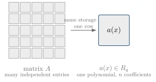
Ring-LWE (Lyubashevsky, Peikert, and Regev, 2010 [2]) replaces that matrix with a single polynomial in a ring \(R_q=\mathbb{Z}_q[x]/(x^n+1)\), shrinking the key from an entire matrix to one row’s worth of coefficients and enabling near-linear-time multiplication. The price is extra algebraic structure, a potential attack surface. This chapter builds RLWE.
Module-LWE (Langlois and Stehlé, 2015 [3]) is the deliberate compromise: a short vector of ring elements instead of a single one. It recovers most of RLWE’s efficiency while diluting the ring structure, hedging against any future attack that exploits the full ring. The next chapter builds it.
ML-KEM (Kyber [4], standardized as FIPS 203 in 2024 [5]) is the module-lattice key-encapsulation mechanism that the next part assembles in full – the destination of this whole progression.
One trade-off runs through the entire story: more algebraic structure buys smaller keys and faster arithmetic, but widens the attack surface. LWE sits at one extreme (no structure, largest keys); RLWE at the other (full ring structure, smallest keys); Module-LWE is the tunable middle that the standard ultimately chose. Note the arc is not monotone – the field advanced to RLWE’s full structure, then deliberately stepped back to Module-LWE as a hedge. With that map in hand, we now build the ring step.
12.2The fatal problem of LWE#
LWE is elegant in theory, but it is not practical in the naive form. Recall the basic equation \[b = A s + e.\] If the dimension is \(n=1024\), then the matrix \(A\) has roughly \(1024\times 1024\) entries, which is more than one million coefficients. If each coefficient is stored in a few bytes, then the public key already becomes large. In practice, a straightforward LWE public key is far too costly for real deployment.
This is why LWE is beautiful theoretically but unattractive in engineering. The algebra is simple, but the representation is bulky.
12.3Observe the negacyclic matrix structure#
RLWE uses the quotient \(x^n+1\), not \(x^n-1\). For \(a(x)=a_0+a_1x+a_2x^2\), multiplication modulo \(x^3+1\) is represented by \[N(a)=\begin{bmatrix} a_0&-a_2&-a_1\\ a_1&a_0&-a_2\\ a_2&a_1&a_0 \end{bmatrix}.\] The shifts are structured, but a coefficient crossing the boundary changes sign because \(x^3=-1\). This is a negacyclic (signed-circulant) matrix, not an ordinary circulant matrix. One polynomial still determines the whole linear map, so the storage benefit remains.
12.4Why negacyclic structure appears#
For \(a(x)=1+2x+3x^2\) and \(s(x)=4+5x+6x^2\), ordinary multiplication creates terms through degree four. Reducing modulo \(x^3+1\) maps \(x^3\) to \(-1\) and \(x^4\) to \(-x\). The sign-flipped wrap-around is the key structure behind RLWE; Chapter 5 develops the cyclic and negacyclic cases side by side.
12.5The working ring \(R_q\)#
RLWE lives not in an ordinary polynomial ring but in the quotient ring \[R_q = \mathbb{Z}_q[x]/(x^n+1),\] whose construction – quotient rings, the reduction rule \(x^n\equiv-1\), and the cyclotomic modulus \(x^n+1\) – was developed in Chapter 4. We recall only what the rest of this chapter needs. Multiplying two polynomials can push the degree to \(n\) or beyond, but the defining relation \(x^n\equiv-1\) (hence \(x^{n+1}\equiv-x\), \(x^{n+2}\equiv-x^2\), and so on) folds every product back to degree below \(n\), so the representation stays compact and structured. Kyber instantiates this as \(R_q=\mathbb{Z}_{3329}[x]/(x^{256}+1)\).
12.6Sage experiment#
We can define a simple quotient ring in Sage.
q = 17
from random import choice
R.<x> = PolynomialRing(GF(q))
S = R.quotient(x^8 + 1)

a = S(x^3 + 2*x + 1)
b = S(x^2 + 3)
print(a*b)
The multiplication is automatically reduced modulo \(x^8+1\).
12.7From LWE to RLWE#
In standard LWE, the secret is a vector \[s=(s_1,\dots,s_n).\] In RLWE, the secret becomes a polynomial \[s(x)=s_0+s_1x+\cdots+s_{255}x^{255}.\] Likewise, the public value \(a\) becomes a polynomial. The noisy equation becomes \[b(x)=a(x)s(x)+e(x).\]
The mathematics is not fundamentally different, but the representation changes. Instead of storing and multiplying large random matrices, we work with structured polynomials. The picture below makes this compression concrete.
12.8Why RLWE is faster#
In ordinary LWE, multiplication is matrix multiplication, which costs roughly \(O(n^2)\) operations. For a dimension around \(256\), this means tens of thousands of operations.
In RLWE, the multiplication is polynomial multiplication. With FFT-like methods, this becomes roughly \(O(n\log n)\). The speedup is substantial. In practice, the ring structure allows the system to run far faster.
This is one of the central reasons RLWE became attractive for real-world deployments.
12.9Fast multiplication via the NTT#
The NTT of Chapter 6 provides the fast representation. A conventional cyclic NTT diagonalizes cyclic convolution; the \(x^n+1\) ring instead needs negacyclic handling. For ML-KEM, the partial NTT maps to 128 quadratic components rather than to unrestricted scalar coordinates. It is this specified transform structure that makes the polynomial products efficient in practice.
12.10Sage experiment: polynomial multiplication#
We can see the basic idea without writing a full NTT implementation.
R.<x> = PolynomialRing(GF(17))
f = 1 + 2*x + x^2
g = 3 + x
print(f*g)
In a full implementation, the NTT (Chapter 6) is the technique used to compute this multiplication much faster than naive schoolbook multiplication.
12.11Is RLWE secure?#
At first glance, the additional algebraic structure might look dangerous. Maybe it makes the problem easier for an attacker. The security story is more subtle. RLWE is based on hardness in ideal lattices, not just general lattices [2]. This makes the security analysis more involved, but it is still believed to be strong enough for practical use.
12.12Sage experiment: a toy RLWE-style setup#
We can create a small ring and form the analog of an LWE sample.
q = 17
from random import choice
R.<x> = PolynomialRing(GF(q))
S = R.quotient(x^8 + 1)

a = S.random_element()  # uniform public ring element

def small_poly():
    return S([choice([-1, 0, 1]) for _ in range(8)])

s = small_poly()
e = small_poly()

b = a*s + e
print("a =", a)
print("s =", s)
print("e =", e)
print("b =", b)
This is a toy RLWE-style sample: \(a\) is uniform, while \(s\) and \(e\) have visibly small coefficients. Written independently of any particular computer-algebra system, the same construction is Algorithm 10.
12.13Comparison: LWE vs RLWE#
| Property | LWE | RLWE |
|---|---|---|
| Data structure | vector and matrix | polynomial |
| Space | \(O(n^2)\) | \(O(n)\) |
| Computation | matrix multiplication | polynomial multiplication |
| Acceleration | limited | NTT-friendly |
| Security foundation | general lattice | ideal lattice |
| Practical deployment | uncommon | widespread |
12.14Why Kyber is not pure RLWE#
A classic interview question is: why is Kyber not pure RLWE? The answer is that Kyber uses a vector of polynomials rather than a single polynomial. In other words, the secret is not just one ring element but a module element over the ring. That is the origin of Module-LWE, which we will study next.
12.15A sibling assumption: NTRU#
RLWE is not the only way to build a hard problem inside the ring \(R_q\). An older construction, NTRU [6] (from 1996, predating LWE), lives in the same ring but hides its secret differently. Instead of the additive-noise equation \(b = a s + e\), NTRU picks two short secret polynomials \(f, g \in R_q\) (with \(f\) invertible) and publishes a single quotient: \[h = g \cdot f^{-1} \pmod q.\] The NTRU assumption is that \(h\) looks like a uniformly random ring element, and that recovering the short pair \((f,g)\) from \(h\) is hard.
q = 17
from random import choice
R.<x> = PolynomialRing(GF(q))
S = R.quotient(x^8 + 1)
def small_unit():
    f = S([choice([-1,0,1]) for _ in range(8)])
    while not f.is_unit():
        f = S([choice([-1,0,1]) for _ in range(8)])
    return f

f = small_unit()              # short and invertible
g = S([0,1,-1,0,1,0,0,-1])   # short
h = g * f^(-1)                # public key
print(h)
There is an equivalent lattice picture, and it is exactly the good-basis/bad-basis story of Part II. The NTRU lattice \[\Lambda = \{ (u,v) \in R_q^2 : u + v\,h \equiv 0 \pmod q \}\] contains the short vector \((g, -f)\), because \(g - f\,h = g - f\,(g/f) = 0\). From \(h\) alone one can only write down a bad (long) basis of \(\Lambda\); the short pair \((f,g)\) is a good basis. Recovering it is a shortest-vector problem in \(\Lambda\).
So RLWE and NTRU are two siblings in the same ring: RLWE hides its secret in additive noise, NTRU hides two short polynomials inside a quotient, and both reduce to finding short vectors in a structured lattice. We single NTRU out here because the FN-DSA signature (Falcon; FIPS 206, still in development, Chapter 18) is built entirely on it.
12.16Summary#
The central idea is simple:
RLWE replaces big random matrices by structured polynomials, which dramatically improves storage and speed while preserving the core noisy linear structure of LWE.
The evolution is:

where the RLWE step is precisely the move to a polynomial ring with negacyclic structure.
Comments