PDF Run this chapter's code LaTeX source Comments

Chapter 3Linear Algebra Foundations

3.1Why this chapter matters#

This chapter is not a general linear algebra course. Its purpose is to develop, with enough precision to be useful later, the specific structures on which post-quantum cryptography is built: vector spaces over a finite field, linear maps and their matrices, and the rank–nullity relationship that governs when a linear system can be solved. The central object of lattice cryptography, the equation \[A\mathbf{s} + \mathbf{e} = \mathbf{b},\] is a linear system deliberately perturbed by a small error \(\mathbf{e}\). To understand why the unperturbed system is easy and the perturbed one is (conjecturally) hard, we first need to be precise about what “solving a linear system” means.

3.2Learning goals#

After reading this chapter, you should be able to:

• state the axioms of a vector space and recognise \(\mathbb{F}_q^n\) as the working example;

• define linear independence, span, basis, and dimension, and know why dimension is well defined;

• describe a matrix as the coordinate form of a linear map, and define its rank, kernel, and image;

• state the rank–nullity theorem and use it to reason about solvability of \(A\mathbf{x}=\mathbf{b}\);

• explain precisely why \(A\mathbf{s}=\mathbf{b}\) is easy while \(A\mathbf{s}+\mathbf{e}=\mathbf{b}\) is the hard LWE problem.

3.3Scalars: the underlying field#

Every vector space is built over a set of scalars that can be added, subtracted, multiplied, and divided. That set is a field (Chapter 2, where the finite field \(\mathbb{F}_q = \mathrm{GF}(q)\) was introduced). We recall the definition because the rest of the chapter depends on it.

The familiar fields are \(\mathbb{Q}\), \(\mathbb{R}\), and \(\mathbb{C}\). Cryptography instead works over the finite field \(\mathbb{F}_q\); for a prime \(q\) this is simply the integers modulo \(q\), \[\mathbb{F}_q = \mathbb{Z}/q\mathbb{Z} = \{0,1,\dots,q-1\},\] with arithmetic reduced modulo \(q\). The property that makes it a field, rather than merely a ring, is that division is available: because \(q\) is prime, every nonzero residue has an inverse. This is exactly what lets Gaussian elimination run, and it is why cryptographic parameters such as \(q=3329\) (Kyber) are chosen prime.

3.4Vectors and vector spaces#

In school a vector is a coordinate tuple such as \((1,2)\). For our purposes a vector is an element of a vector space: a structured container of field elements that can be added and scaled.

A typical secret is written \[\mathbf{s} = \begin{bmatrix}2\\5\\1\\7\end{bmatrix} \in \mathbb{F}_{q}^{4}, \qquad\text{or in practice}\qquad \mathbf{s} \in \mathbb{F}_{3329}^{256}.\]

3.4.1Sage experiment: creating a vector#

F = GF(17)
v = vector(F, [1, 2, 3])
v

To inspect its type, use type(v). Sage reports it as a free module element rather than a plain list. This is not pedantry: a vector space over a field is the special case of a module over a ring in which the ring happens to be a field, and Module-LWE (Chapter 13) will use exactly the more general object.

3.4.2Vector addition and scalar multiplication#

a = vector(F, [1, 2, 3])
b = vector(F, [5, 6, 7])
a + b        # (6, 8, 10)
3 * a        # (3, 6, 9)

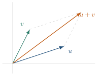
All arithmetic is modulo the field characteristic: over \(\mathbb{F}_7\) the sum \(6+5\) is \(4\), not \(11\). Over \(\mathbb{R}\) or \(\mathbb{Q}\) addition has the familiar parallelogram picture of Figure 3.1.

3.5Linear combinations, independence, and span#

The single most important operation in the whole subject is forming a linear combination.

For instance \((1,0)\) and \((0,1)\) are independent, whereas \((1,2)\) and \((2,4)\) are dependent, since the second is twice the first.

3.5.1Sage experiment: detecting dependence through rank#

Dependence is detected numerically by rank, defined precisely below: stacking the vectors as rows, the rank counts how many are genuinely independent.

A = Matrix(GF(17), [[1, 2], [2, 4]])
A.rank()      # 1: only one independent direction

3.6Basis and dimension#

The standard basis of \(\mathbb{F}_q^2\) is \(\{(1,0),(0,1)\}\), since \((a,b)=a(1,0)+b(0,1)\). But \(\{(2,1),(1,1)\}\) is an equally valid basis of the same space: the space is intrinsic, the basis is a chosen coordinate system for it. The number of vectors in a basis is not a matter of choice.

Thus \(\dim \mathbb{F}_q^n = n\). The freedom to change basis without changing the space is the seed of the entire theory of lattice reduction (Chapter 8): a lattice, too, has many bases, and finding a good one is the central algorithmic problem.

3.6.1Sage experiment: two bases for one space#

B1 = Matrix(GF(17), [[1, 0], [0, 1]])
B2 = Matrix(GF(17), [[2, 1], [1, 1]])
# both have rank 2, so each is a basis of GF(17)^2
print(B1.rank(), B2.rank())

3.7Matrices as linear maps#

A matrix is best understood not as a grid of numbers but as the coordinate form of a linear map.

The product \(A\mathbf{v}\) is itself a linear combination: it is the combination of the columns of \(A\) weighted by the entries of \(\mathbf{v}\). Concretely, entry \(i\) of the result is the inner product of row \(i\) of \(A\) with \(\mathbf{v}\), which is exactly the double loop of Algorithm 2.

F = GF(17)
A = Matrix(F, [[1, 2], [3, 4]])
v = vector(F, [5, 6])
A * v

This same loop is foundational for the whole book: it computes \(A\mathbf{s}\) in the LWE equation, and in ring form (Chapter 12) it reappears as the schoolbook polynomial multiplication used by RLWE and Kyber.

3.8Rank, kernel, and image#

Three subspaces measure what a linear map \(A\colon\mathbb{F}^n\to\mathbb{F}^m\) does.

The image is exactly the set of right-hand sides \(\mathbf{b}\) for which \(A\mathbf{x}=\mathbf{b}\) has a solution. The kernel measures how far a solution is from unique: if \(A\mathbf{x}_0=\mathbf{b}\), then the full solution set is \(\mathbf{x}_0 + \ker A\). These two dimensions are tied together.

In particular, a square matrix \(A\in\mathbb{F}^{n\times n}\) is invertible if and only if its rank is \(n\), equivalently \(\ker A=\{\mathbf{0}\}\), equivalently its columns are a basis of \(\mathbb{F}^n\). When \(A\) is invertible, \(A\mathbf{x}=\mathbf{b}\) has exactly one solution for every \(\mathbf{b}\).

3.8.1Sage experiment: rank governs invertibility#

F = GF(17)
for _ in range(10):
    A = random_matrix(F, 4, 4)
    print(A.rank())

For a uniformly random \(n\times n\) matrix over \(\mathbb{F}_q\), the invertibility probability is \[\prod_{i=1}^{n}(1-q^{-i}).\] Thus the claim depends on \(q\): for this \(4\times4\) example over \(\mathbb{F}_{17}\) it is high, while over \(\mathbb{F}_2\) it is only about \(30.8\%\).

3.9Solving linear systems, and the leap to LWE#

Given \(A\) and \(\mathbf{b}\), the equation \(A\mathbf{x}=\mathbf{b}\) is solved by Gaussian elimination: row operations reduce \(A\) to echelon form, and back-substitution recovers \(\mathbf{x}\).

This efficiency is precisely why a plain linear system carries no cryptographic value: anyone who sees \(A\) and \(\mathbf{b}=A\mathbf{s}\) can recover the secret \(\mathbf{s}\) in cubic time. LWE changes the setting. Given a public, typically rectangular random matrix \(A\in\mathbb{Z}_q^{m\times n}\) with \(m>n\), a secret \(\mathbf{s}\) drawn from a prescribed small distribution, and an independent small error vector \(\mathbf{e}\), one observes samples \[\mathbf{b} = A\mathbf{s} + \mathbf{e},\] with arithmetic modulo \(q\). Unlike an invertible square system, this overdetermined system will generally have no exact solution for a nonzero random error. Gaussian elimination can detect inconsistency, but it does not recover the planted secret from the noisy samples. Recovering \(\mathbf{s}\) is the Learning With Errors problem (Chapter 11).

3.10Experiments#

F = GF(17)
# 1. random vectors
V = VectorSpace(F, 4)
for _ in range(5): print(V.random_element())

# 2. a matrix acting on a vector
A = random_matrix(F, 6, 4); v = random_vector(F, 4)
print(A * v)

# 3. exact solve is easy; try recovering s from b = A*s
s = random_vector(F, 4); b = A * s
print(A.solve_right(b) == s)   # True when A has full column rank

# 4. perturb an overdetermined system: it normally becomes inconsistent
e = vector(F, [1, 0, 0, 16, 0, 0])   # 16 == -1 mod 17
try:
    A.solve_right(b + e)
except ValueError:
    print("no exact solution: noisy samples are inconsistent")

The experiment is a toy illustration only: real LWE specifies the dimensions and the secret and error distributions precisely.

3.11Connection to the next chapter#

The next chapter, Polynomial Rings, keeps the linear-algebraic viewpoint but changes the scalars-and-vectors picture into a single richer object. A structured (circulant) matrix will be encoded by one polynomial, matrix–vector multiplication will become polynomial multiplication, and the vector space \(\mathbb{F}_q^n\) will be upgraded to the quotient ring \[R_q = \mathbb{Z}_q[x]/(x^n + 1),\] the natural home of RLWE and Kyber.