PDF Run this chapter's code LaTeX source Comments
Chapter 16Complete Implementation of ML-KEM (FIPS 203)
16.1Learning objectives#
This chapter assembles the pieces built earlier in the book – the negacyclic ring and the NTT (Chapter 6), the toy scheme (Chapter 14), and centered binomial sampling (Chapter 15) – into the real standard. FIPS 203, ML-KEM (from the submission CRYSTALS-Kyber) [1, 2], is the module-lattice-based key-encapsulation standard, and the first of NIST’s post-quantum standards to be finalized (2024). All algorithm and data-flow details in this chapter follow FIPS 203 [1].
After finishing this chapter, you should be able to:
follow the full ML-KEM key generation workflow and its data types at every stage;
explain why key generation is almost entirely deterministic once the initial seed is fixed;
follow encapsulation and explain why a KEM encapsulates a random secret rather than encrypting chosen data;
follow decapsulation and explain the Fujisaki–Okamoto “re-encrypt and compare” transform with implicit rejection;
distinguish the CPA-secure inner scheme (K-PKE) from the CCA-secure KEM (ML-KEM) built on top of it.
16.2Review: Toy Kyber versus real ML-KEM#
In the toy implementation of Chapter 14, we used the following informal key-generation pattern:
\[A \xleftarrow{\$} R_q^{k\times k}, \qquad s,e \xleftarrow{\$} \chi, \qquad t = A\cdot s + e.\]
The output was then a key pair \((pk, sk)\).
The most important difference is that all random objects were generated directly and independently.
In real ML-KEM, this is not the case. The algorithm starts from a short random seed and then deterministically expands the rest of the randomness from it.
16.3The real input in FIPS 203#
The standard key generation procedure does not begin by generating a matrix at random. It begins by generating a short random seed:
\[d \in \{0,1\}^{256}.\]
In other words, the input to the standard algorithm is a 256-bit seed. We can think of the whole key generation algorithm as a deterministic function
\[\mathrm{KeyGen}(d)\]
rather than as a random process that samples all objects independently.
This is the first major conceptual shift from toy Kyber to the real standard.
16.4Phase 1: expand the seed#
The first step in the standard is to compute
\[(\rho, \sigma) = G(d),\]
where:
\(\rho\) is used to generate the matrix \(A\);
\(\sigma\) is used to generate the secret and error polynomials.
In the standard, \(G\) is built from SHA3-512. In a teaching implementation, we can first abstract it as a black box:
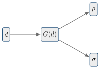
The pedagogical point is that the entire randomness of the later steps is derived from the initial seed \(d\).
16.5Phase 2: generate the matrix#
The matrix is not stored as a random object in the public key. Instead, it is reconstructed from a seed:
\[A = \mathrm{ExpandA}(\rho).\]
This is a deterministic map:
\[\mathrm{ExpandA}: \{0,1\}^{256} \to R_q^{k\times k}.\]
The same seed always yields the same matrix. This is a crucial compression trick in the standard.
SageMath experiment#
For a teaching implementation, we can first simulate the expansion by using a simple deterministic pseudo-random generator.
from random import Random
from sage.all import GF, Matrix, PolynomialRing

q = 17
n = 8
k = 2
R.<x> = PolynomialRing(GF(q))
Rq = R.quotient(x^n + 1)


def expand_A(seed):
    rng = Random(str(seed))
    return Matrix(
        Rq,
        k,
        k,
        [Rq([rng.randrange(q) for _ in range(n)])
         for _ in range(k * k)]
    )
The important thing is not the exact random source at this stage. The important thing is the interface:
same seed \(\Rightarrow\) same matrix;
different seed \(\Rightarrow\) different matrix.
16.6Phase 3: generate the secret vector#
The secret vector is derived from the CBD distribution. In other words,
\[s \leftarrow \mathrm{CBD}(\sigma).\]
This is not uniform sampling. The coefficients are small integers sampled from a centered binomial distribution. Each coefficient of the secret polynomial is therefore a small signed value rather than an arbitrary element of the ring.
The secret vector is therefore a vector of small polynomials:
\[s = (s_0, \dots, s_{k-1}).\]
16.7Phase 4: generate the error vector#
The error vector is generated in a very similar way, again using CBD-based sampling:
\[e \leftarrow \mathrm{CBD}(\sigma).\]
The exact detail depends on the parameter set, but the conceptual point is the same: the noise is derived from a short seed through a deterministic sampling procedure.
16.8Phase 5: compute the public key in the NTT domain#
FIPS 203 samples the secret and error in coefficient form, then transforms them. ExpandA already produces the matrix in the NTT representation. The public vector is computed as \[\hat t=\hat A\circ\hat s+\hat e,\] where \(\circ\) uses the specified MultiplyNTTs operation: 128 quadratic base products, not unrestricted coordinate-wise scalar multiplication. The PKE public key encodes \((\hat t,\rho)\) and the PKE secret key encodes \(\hat s\); an inverse NTT is used later where coefficient-domain values are required. This is the data flow of FIPS 203, Sections 4.3.1 and 5.1.
16.9Phase 7: encode the public key#
The real public key is not the pair \((A,t)\). Instead, it is essentially the pair
\[(\rho, t).\]
The reason is that the matrix \(A\) can be regenerated from the seed \(\rho\). Therefore the public key stores only what is truly necessary:
the seed \(\rho\);
the vector \(t\).
16.10KeyGen data flow#
The whole process can be summarized as follows:
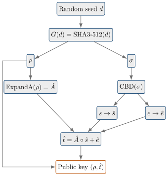
This flow should be remembered because it reappears inside encapsulation and decapsulation below. Written as pseudocode, the seven phases above collapse into a single short algorithm:
Every line here is deterministic given \(d\); the only place fresh randomness enters the entire computation is the sampling of \(d\) itself.
16.11From K-PKE to ML-KEM: the two layers#
The algorithm above is not quite ML-KEM. It is the key generation of K-PKE, the underlying public-key encryption scheme, which is only CPA-secure – safe against a passive eavesdropper, but not against an attacker who submits chosen ciphertexts and watches how decryption responds. ML-KEM is K-PKE wrapped in one more layer. K-PKE provides three routines, \[\text{K-PKE.K}{\small\text{EY}}\text{G}{\small\text{EN}},\qquad \text{K-PKE.E}{\small\text{NCRYPT}}(ek, m, r),\qquad \text{K-PKE.D}{\small\text{ECRYPT}}(dk, c),\] and the Fujisaki–Okamoto (FO) transform [3] turns them into a CCA-secure key-encapsulation mechanism. ML-KEM key generation simply calls K-PKE key generation and stores a little extra in the secret key:
The encapsulation key \(ek=(\rho,t)\) is what a KEM publishes. The decapsulation key carries the PKE secret \(dk_{\mathrm{PKE}}=s\), a copy of \(ek\) and its hash \(H(ek)\) (both needed to re-encrypt during decapsulation), and the random value \(z\) whose role becomes clear below.
16.12Encapsulation#
Encapsulation produces a fresh shared secret \(K\) and a ciphertext \(c\) from which the holder of \(dk\) can recover the same \(K\). The design choice that defines a KEM – and the answer to “why encapsulate a random secret instead of encrypting a chosen message?” – is that the encrypted message is not chosen by the sender at all. Encapsulation samples a random \(32\)-byte value \(m\), and derives both the shared key and the encryption randomness by hashing it. That the randomness is a deterministic function of the message is exactly what the FO transform will exploit.
Inside \(\text{K-PKE.E}{\small\text{NCRYPT}}\) the message is hidden in the same noisy-linear way as the toy scheme of Chapter 14, now driven by the seed \(r\): the matrix is regenerated as \(A=\text{E}{\small\text{XPAND}}\text{A}(\rho)\), small vectors \(y,e_1,e_2\) are sampled from CBD using \(r\), and the ciphertext is the compressed pair \[u = A^{T} y + e_1, \qquad v = t^{T} y + e_2 + \mathrm{Encode}(m).\] The shared secret \(K\) itself never travels on the wire; only \(c\) does, and the recipient reconstructs \(K\) from it.
16.13From CPA to CCA: the Fujisaki–Okamoto transform#
Everything built so far – the toy scheme of Chapter 14, the real noise of Chapter 15, and K-PKE above – is a public-key encryption scheme secure only against a passive eavesdropper. One more layer is needed before any of it is safe to deploy, and FIPS 203 is blunt that the layer is not optional: K-PKE “is not IND-CCA2-secure and shall not be used as a stand-alone scheme” [1]. This section explains what that missing property is and how the Fujisaki–Okamoto (FO) transform supplies it. The same transform reappears in every other KEM in this book – Classic McEliece (Chapter 22), HQC (Chapter 23), and SIKE (Chapter 25) – so it is worth meeting properly once.
Two attack models.#
Security notions for encryption differ in what the attacker may do, not in what they are trying to learn. Under both notions the attacker picks two messages, is given an encryption of one of them, and must say which:
IND-CPA – indistinguishability under chosen-plaintext attack. The attacker holds the public key and so can encrypt anything they wish. This models a passive eavesdropper.
IND-CCA2 – indistinguishability under adaptive chosen-ciphertext attack. The attacker may additionally submit ciphertexts of their own construction to the honest key holder and observe the result, both before and after seeing the challenge; only decrypting the challenge itself is barred.
The distance between the two is the distance between an attacker who listens and one who interacts. Real protocols grant the second kind of access almost by definition: a server decrypts whatever arrives on the wire, and what it does next – an error, a timing difference, a retry – is visible to whoever sent it.
Why the passive scheme breaks.#
The failure is concrete rather than theoretical. A K-PKE ciphertext is a pair \((\mathbf{u}, v)\) in which the message bits are carried by \(v\), each scaled by \(\lceil q/2 \rceil\). Arithmetic is coordinatewise, so an attacker who intercepts \((\mathbf{u}, v)\) and forwards \((\mathbf{u},\ v + \lceil q/2 \rceil)\) hands the receiver a perfectly valid ciphertext that decrypts to the complement of the original message – without knowing the secret key and without ever learning the message. This is malleability: ciphertexts can be edited into related ciphertexts. The linearity that makes lattice encryption fast is exactly what makes it malleable.
The decryption oracle leaks, too. Feed the key holder a stream of slightly malformed ciphertexts and record which decrypt cleanly; each answer is one inequality constraining the secret, and enough of them recover it. This is why a passively secure lattice scheme must never be exposed directly.
The key idea: make encryption deterministic.#
Malleability survives only because a ciphertext carries no evidence of how it was built. Encryption is randomized – \(\text{E}{\small\text{NCRYPT}}(ek, m; r)\) for a fresh random \(r\) – so a message has many valid ciphertexts and the receiver cannot tell an honest one from a doctored one.
FO removes the freedom. Rather than sampling \(r\), derive it from the message: \(r = G(m)\). Encryption becomes a function of the message alone, so each message now has exactly one valid ciphertext – and that makes ciphertexts checkable. The receiver decrypts to a candidate \(m'\), recomputes the ciphertext that \(m'\) must have produced, and compares. An honest ciphertext matches; anything the attacker altered does not.
The KEM setting is what makes this painless. Because a KEM transports a random secret rather than a chosen message (Chapter 14), deriving the randomness from the message costs nothing – the message was never the point. Encapsulation samples a random \(m\) and hashes it into both the shared key and the encryption randomness, which is precisely what Algorithm 18 does with \((K, r) \gets G(m \,\|\, h)\).
The transform in two steps.#
The modern presentation, due to Hofheinz, Hövelmanns, and Kiltz [4] and cited by FIPS 203 itself, splits FO into two independent pieces:
the \(T\) transform derandomizes, turning an IND-CPA encryption scheme into a deterministic one whose ciphertexts can be validated by re-encryption;
the \(U\) transform wraps that deterministic scheme into a KEM, deriving the shared secret by hashing and deciding what to do when the re-encryption check fails.
Separating the two is what lets the security proof be assembled from parts, and it is why the literature speaks of a family of FO variants rather than one algorithm. ML-KEM uses one specific member of that family, which the next section spells out.
16.14Decapsulation and the Fujisaki–Okamoto transform#
Decapsulation must recover \(K\) from \(c\) using \(dk\), and – this is the entire point of the FO transform – it must do so in a way that gives an attacker no usable signal from submitting malformed ciphertexts. The mechanism is re-encrypt and compare: decrypt to a candidate message, deterministically re-run encapsulation from it, and check that the ciphertext that would have been produced matches the one received.
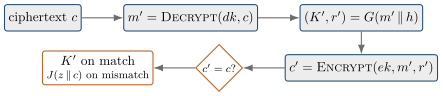
The subtlety is the else branch. A naive KEM would return an error on a bad ciphertext – but that error is an oracle: by observing whether decapsulation succeeds, an attacker can mount a chosen-ciphertext attack and, over many queries, extract the secret. Implicit rejection closes this door: on a mismatch, ML-KEM returns a pseudorandom key \(J(z\,\|\,c)\) derived from the secret \(z\), of exactly the same form as a real key. Success and failure become indistinguishable to the caller, so there is no oracle. This is what lifts K-PKE from CPA to IND-CCA2 security; it is why the comparison \(c'=c\) must run in constant time (Chapter 26); and it is the same mechanism the code-based KEM HQC uses (Chapter 23).
Explicit versus implicit rejection.#
The two ways of handling a failed comparison name the two branches of the FO family. Explicit rejection returns a distinguished error symbol \(\bot\); implicit rejection returns a pseudorandom key, as ML-KEM does. Implicit rejection is the more conservative choice on three counts: it removes the error signal outright instead of trusting every caller to handle \(\bot\) safely; it keeps decapsulation a single straight-line computation, which is far easier to make constant-time; and it is the variant for which the tightest security proofs against quantum adversaries are known (Section 16.16).
One detail of ML-KEM’s particular variant is easy to miss. The hash \(h = H(ek)\) of the encapsulation key is fed into \(G\) alongside the message, binding the shared secret to the public key it was produced under. FIPS 203 also departs here from the third-round Kyber submission: encapsulation no longer hashes the ciphertext into the shared secret [1]. That change is safe precisely because the re-encryption check already ties the ciphertext to the message.
16.15Decryption failures#
Re-encrypt-and-compare assumes decryption returns the message that was encrypted. For lattice schemes that is only almost always true. The noise of Chapter 15 can, with small probability, push a coefficient past a rounding boundary and flip a bit of \(m'\); the recomputed ciphertext then fails to match and decapsulation returns the wrong key. This is a correctness failure, not an attack, and FIPS 203 tabulates its probability [1]:
| Parameter set | Decapsulation failure rate |
|---|---|
| ML-KEM-512 | \(2^{-138.8}\) |
| ML-KEM-768 | \(2^{-164.8}\) |
| ML-KEM-1024 | \(2^{-174.8}\) |
These numbers are not merely about reliability. A decryption failure is a leak: it happens only for ciphertexts whose noise correlates with the secret key, so an attacker able to find failing ciphertexts learns something about \(\mathbf{s}\), and the FO security bound degrades as the failure rate climbs. That is why the rate is driven far below anything a user would ever notice, and why parameter selection treats it as a security quantity rather than an engineering tolerance. Attacks on earlier LWE-based designs such as LAC show how attacker-shaped ciphertexts and observable failure events can turn that correlation into a practical oracle [5]; malformed inputs, timing, and retry behaviour must not reveal which internal check failed.
16.15.1Compression beyond ML-KEM#
ML-KEM already compresses polynomial coefficients by quantization. More aggressive research proposals treat a ciphertext as a structured communication signal and use lattice coding or packing, including in multi-recipient settings [6]. This is not ordinary lossless compression: the decoder, noise distribution, failure probability, decapsulation cost, and chosen-ciphertext proof all change together. A size claim is therefore incomplete unless it reports transmitted bytes, decoder work and memory, the failure probability under the actual noise model, and any additional assumption introduced by packing recipients together.
16.16The random oracle model, and its quantum version#
The FO proof rests on an explicit assumption, stated in FIPS 203 itself: the analysis holds “under the heuristic assumption that hash functions and XOFs behave like uniformly random functions” [1]. This is the random oracle model (ROM). In it, \(G\), \(H\), and \(J\) are replaced by genuinely random functions that every party – honest or hostile – can only query as a black box. The model is a heuristic, and knowingly so: SHA3-512 is a fixed public algorithm, not a random function. But proofs in it have been a reliable guide in practice, and no break of a deployed scheme has yet been traced to the gap.
For post-quantum cryptography the heuristic needs a second look, and here the story becomes specific to this book’s subject. A quantum attacker does not query SHA3 as a black box. The function is public, so the attacker can build the circuit and evaluate it on a superposition of inputs, extracting information about many outputs at once. Modelling that faithfully requires the quantum random oracle model (QROM), introduced by Boneh and co-authors [7], in which oracle queries may themselves be superpositions.
The distinction is not pedantry, because classical ROM proofs do not automatically survive the move. A great many of them work by watching the attacker’s queries and reading off the useful one – the reduction simply observes which \(m\) the attacker hashed. Against superposition queries that step is illegitimate: measuring a quantum query disturbs it. Re-establishing FO security in the QROM was therefore a research programme in its own right, beginning with the modular analysis of Hofheinz, Hövelmanns, and Kiltz [4] and continuing through a line of increasingly tight bounds for the implicit-rejection variant [8].
This is the honest reason FIPS 203 claims only that ML-KEM “is believed to satisfy so-called IND-CCA2 security” [1]. The lattice assumption is one source of doubt; the random oracle heuristic, in its quantum form, is a second and quite independent one. If a reader takes one thing from this section, it should be that “provably secure” always carries a model with it – and that for every KEM in this book, that model includes a hash function idealized in a way no real hash function is.
16.17Parameter sets#
| Scheme | \(k\) | \(\eta_1\) | \((d_u,d_v)\) | NIST level | Comparable to |
|---|---|---|---|---|---|
| ML-KEM-512 | 2 | 3 | \((10,4)\) | 1 | AES-128 |
| ML-KEM-768 | 3 | 2 | \((10,4)\) | 3 | AES-192 |
| ML-KEM-1024 | 4 | 2 | \((11,5)\) | 5 | AES-256 |
16.18SageMath experiments#
The most useful way to study this chapter is through three short experiments.
Experiment 1: verify ExpandA#
Use the same seed twice:
A1 = expand_A(1234)
A2 = expand_A(1234)
Then verify that \(A_1 = A_2\). Now change the seed and observe that the matrix changes as well.
Experiment 2: inspect CBD statistics#
Generate many samples from the CBD distribution and check that the average is close to zero.
from random import randint

def cbd(eta):
    return sum(randint(0, 1) for _ in range(eta)) - \
           sum(randint(0, 1) for _ in range(eta))

samples = [cbd(2) for _ in range(10000)]
print(sum(samples) / len(samples))
Observe how the variance changes when \(\eta\) changes.
Experiment 3: implement a teaching version of key generation#
Finally, write a function
pk, sk = keygen(seed)and test the following properties:
same seed gives the same key pair;
different seeds give different key pairs.
This gives a first impression of how modern public-key cryptography is built from deterministic pseudo-random procedures.
Experiment 4: one MultiplyNTTs base product#
The NTT-domain multiplication in FIPS 203 is not 256 independent scalar products. Each coordinate pair is multiplied modulo a quadratic relation. The following check implements one such pair; it tests the algebraic base case, not the full standardized transform or its serialization.
q = 3329

def multiply_ntt_pair(a, b, gamma):
    a0, a1 = a
    b0, b1 = b
    return ((a0*b0 + gamma*a1*b1) % q,
            (a0*b1 + a1*b0) % q)

# (1 + 2X)(3 + 4X) modulo X^2 - gamma, with gamma = 17.
got = multiply_ntt_pair((1, 2), (3, 4), 17)
assert got == ((3 + 17*8) % q, (4 + 6) % q)
print("one ML-KEM quadratic base product:", got)
This is precisely the local multiplication used 128 times by MultiplyNTTs; a conforming ML-KEM implementation must additionally use FIPS 203’s transform ordering, twiddle factors, reductions, encodings, and test vectors.
16.19A complete SageMath implementation#
The experiments above illustrate individual pieces. The companion file sage/fips203_mlkem.sage assembles all of them into a complete, byte-exact implementation of FIPS 203: every one of the standard’s twenty-one numbered algorithms appears as its own function, named after the standard and annotated with its algorithm number, for all three parameter sets.
Run it in a browser: every algorithm in this chapter, at all three parameter sets. See appliedpqc.io/playground.html — nothing to install.
The algebraic objects are genuine Sage objects rather than opaque byte arrays. The coefficient domain is the quotient ring itself, \[R_q = \mathbb{Z}_q[X]/(X^{256}+1),\] and the NTT domain \(T_q\) is carried as a Sage vector over \(\mathbb{F}_q\):
MLKEM_n, MLKEM_q, MLKEM_zeta = 256, 3329, 17

Fq = GF(MLKEM_q)
Rx = PolynomialRing(Fq, 'X')
X  = Rx.gen()
Rq = Rx.quotient(X^MLKEM_n + 1, 'x')   # coefficient domain
Tq = VectorSpace(Fq, MLKEM_n)          # NTT domain

ZETA  = [Fq(MLKEM_zeta)^BitRev7(i) for i in range(128)]
GAMMA = [Fq(MLKEM_zeta)^(2*BitRev7(i) + 1) for i in range(128)]
With that in place, the transform is the standard’s butterfly network written directly over \(\mathbb{F}_q\):
def NTT(f):
    """Algorithm 9. Map f in Rq to its NTT representation in Tq."""
    fh = _coeffs(f)
    i, length = 1, 128
    while length >= 2:
        for start in range(0, MLKEM_n, 2*length):
            z = ZETA[i]; i += 1
            for j in range(start, start + length):
                t = z * fh[j + length]
                fh[j + length] = fh[j] - t
                fh[j]          = fh[j] + t
        length //= 2
    return vector(Fq, fh)
Key generation is then the seven phases of this chapter, line for line:
def KPKE_KeyGen(self, d):
    """Algorithm 13. K-PKE.KeyGen(d) -> (ek_PKE, dk_PKE)."""
    k = self.k
    rho, sigma = _G(bytes(d) + bytes([k]))   # domain separator k
    N = 0
    Ah = self._ExpandA(rho)
    s = []
    for _ in range(k):
        s.append(SamplePolyCBD(self.eta1, _PRF(self.eta1, sigma, N))); N += 1
    e = []
    for _ in range(k):
        e.append(SamplePolyCBD(self.eta1, _PRF(self.eta1, sigma, N))); N += 1
    sh = [NTT(si) for si in s]
    eh = [NTT(ei) for ei in e]
    th = [ntt_vec_dot(Ah[i], sh) + eh[i] for i in range(k)]
    ek = b"".join(ByteEncode(12, _ints(t)) for t in th) + rho
    dk = b"".join(ByteEncode(12, _ints(si)) for si in sh)
    return ek, dk
Note the byte k appended to the seed in the very first line: FIPS 203 domain-separates the three parameter sets so that a seed expanded under the wrong one yields an unrelated key.
Why a computer-algebra system earns its place here.#
Because \(R_q\) is a real Sage ring, the hand-rolled transform can be checked against the algebra it claims to implement rather than merely against itself. The function verify_ntt_is_a_ring_isomorphism(), defined at the end of sage/fips203_mlkem.sage, confirms three things using Sage’s own arithmetic as the oracle: that \(\mathrm{NTT}^{-1}\) inverts \(\mathrm{NTT}\); that the \(i\)-th output coefficient pair really is \(f \bmod (X^2-\gamma_i)\), so the transform is the Chinese-remainder map onto the \(128\) quadratic factors of \(X^{256}+1\); and that \[\mathrm{NTT}(f\cdot g) \;=\; \text{M}{\small\text{ULTIPLY}}\text{NTT}{\small\text{S}}\big(\mathrm{NTT}(f),\,\mathrm{NTT}(g)\big),\] where the left-hand product is computed by Sage in \(R_q\). That last identity is precisely the statement that the NTT is a ring isomorphism \(R_q \to T_q\) – the fact the single-base-product check earlier in this chapter could only gesture at.
Validation.#
Correctness is not argued, it is measured. The test runner sage/test_kat.sage checks the implementation against NIST’s ACVP test vectors [10], which carry both the inputs and the expected outputs of every case: key generation, encapsulation, decapsulation, and the encapsulation- and decapsulation-key validity checks of Sections 7.2 and 7.3. All outputs match byte for byte across ML-KEM-512, 768, and 1024. From the book’s latex/ directory, make kat runs it.
16.20Pitfalls#
Pitfall 1: thinking that the matrix \(A\) is stored explicitly#
This is not true in the standard. The matrix is derived from \(\rho\) and therefore regenerated when needed.
Pitfall 2: thinking that CBD is truly random sampling#
CBD is not random sampling in the naive sense. It is a deterministic sampling procedure driven by a seed and an expansion function.
Pitfall 3: thinking that KeyGen calls the random generator at every step#
In the real algorithm, the initial seed \(d\) is the only place where fresh randomness is introduced. Everything after that is a deterministic transform.
Pitfall 4: returning an error on decryption failure#
An implementation that signals “bad ciphertext” instead of returning the implicit-rejection key \(J(z\,\|\,c)\) reintroduces a decryption-failure oracle and breaks CCA security. Both the comparison \(c'=c\) and the choice between \(K'\) and \(J(z\,\|\,c)\) must be constant-time.
16.21Summary#
ML-KEM is a two-layer construction, and this chapter built it end to end:
the inner K-PKE is a CPA-secure public-key encryption whose entire key generation is a deterministic expansion of one seed, \[d \longrightarrow (\rho,\sigma) \longrightarrow (A,s,e) \longrightarrow t \longrightarrow (\rho,t),\] publishing only \((\rho,t)\) and never \(A\);
encapsulation hides a random message \(m\), deriving both the shared key \(K\) and the encryption randomness \(r\) by hashing \(m\), so the ciphertext is a deterministic function of \(m\);
decapsulation decrypts, re-encrypts, and compares – returning the real key on a match and a pseudorandom key \(J(z\,\|\,c)\) on a mismatch. This is the Fujisaki–Okamoto transform with implicit rejection, and it is what lifts CPA security to IND-CCA2.
That completes the first NIST post-quantum standard, FIPS 203, from a single random seed to a CCA-secure shared key. The next part turns from key establishment to the other half of public-key cryptography – digital signatures – beginning with the lattice-based standards ML-DSA and FN-DSA, which reuse much of the machinery (module lattices, CBD sampling, the NTT) built here.
Comments