PDF Run this chapter's code LaTeX source Comments

Chapter 4Polynomial Rings

4.1Why this chapter matters#

The previous chapter expressed cryptographic objects as vectors and matrices over a field. This chapter changes the algebra: instead of a vector space \(\mathbb{F}_q^n\) we work in a quotient polynomial ring \[R_q = \mathbb{Z}_q[x]/(x^n+1),\] the setting of RLWE, Kyber, and Dilithium. The payoff is structural. A single element of \(R_q\) carries the same information as a whole structured \(n\times n\) matrix, and multiplication in \(R_q\) is a form of convolution that admits a fast transform (the NTT of Chapter 6). To use this ring safely we need to be precise about what it is: what a ring is, what a quotient by a polynomial means, and why the particular modulus \(x^n+1\) is chosen.

4.2Learning goals#

After reading this chapter, you should be able to:

state what a (commutative) ring is and recognise \(\mathbb{F}_q[x]\) as one;
perform Euclidean division of polynomials and explain why it makes quotient rings well defined;
construct the quotient ring \(\mathbb{F}_q[x]/(f)\) and count its elements;
state when the quotient is a field, and why \(x^n+1\) (for \(n\) a power of two) is the natural modulus;
describe multiplication in \(R_q\) as negacyclic convolution and connect it to the NTT.

4.3Rings and fields#

A field, from Chapter 3, supports addition, subtraction, multiplication, and division. A ring is the weaker structure in which division may fail.

Definition 4.1 (Commutative ring). A commutative ring with identity is a set \(R\) with operations \(+\) and \(\cdot\) such that \((R,+)\) is an abelian group with identity \(0\), multiplication is associative and commutative with an identity \(1\), and multiplication distributes over addition. A field is the special case in which every nonzero element has a multiplicative inverse.

The integers \(\mathbb{Z}\) form a ring but not a field (\(2\) has no integer inverse); the integers modulo a prime, \(\mathbb{F}_q\), form a field. The distinction matters here because we will build new rings out of polynomials, and those are generally not fields.

4.4The polynomial ring \(\mathbb{F}_q[x]\)#

Definition 4.2 (Polynomial ring). For a field \(\mathbb{F}\), the polynomial ring \(\mathbb{F}[x]\) consists of all finite expressions \[f(x) = a_0 + a_1 x + \cdots + a_d x^d,\qquad a_i\in\mathbb{F},\] with addition and multiplication of polynomials. The degree \(\deg f\) is the largest \(i\) with \(a_i\neq 0\). It is a commutative ring with identity \(1\).

A polynomial is, coefficient by coefficient, just a vector: \(f(x)=3x^4+2x^2+5\) is the coefficient list \((5,0,2,0,3)\). Addition of polynomials is addition of these coefficient vectors. The new ingredient is multiplication, and it is not entrywise.

Proposition 4.3 (Multiplication is convolution). If \(f(x)=\sum_i a_i x^i\) and \(g(x)=\sum_j b_j x^j\), then \[(fg)(x) = \sum_{k} c_k x^k, \qquad c_k = \sum_{i+j=k} a_i b_j.\] The coefficient sequence \((c_k)\) is the convolution of \((a_i)\) and \((b_j)\).

For example \((x+1)(x+2)=x^2+3x+2\), where the middle coefficient \(3=1\cdot 2+1\cdot 1\) is a sum of cross terms. This convolution is the operation that the NTT will later accelerate.

4.4.1Sage experiment: the polynomial ring#

F = GF(17)
R.<x> = PolynomialRing(F)
f = 3*x^4 + 2*x^2 + 5
print(f.degree())        # 4
print(f.list())          # [5, 0, 2, 0, 3]: the coefficient vector
print((x+1)*(x+2))       # x^2 + 3*x + 2

4.5Euclidean division#

The one structural fact that makes everything below work is that polynomials over a field can be divided with remainder, exactly like integers.

Theorem 4.4 (Division algorithm in \(\mathbb{F}[x]\)). For \(f,g\in\mathbb{F}[x]\) with \(g\neq 0\) there exist unique polynomials \(q\) (quotient) and \(r\) (remainder) with \[f = q\,g + r, \qquad \deg r < \deg g.\]

Uniqueness of the remainder is what will let us reduce every polynomial modulo a fixed \(g\) to a single canonical form of degree below \(\deg g\). That canonical form is the coefficient vector we actually store.

4.6Quotient rings#

Left unbounded, degrees grow without limit under multiplication. We tame this by declaring a fixed polynomial to be zero.

Definition 4.5 (Ideal and quotient ring). The principal ideal generated by \(f\in\mathbb{F}[x]\) is the set of all multiples \((f)=\{f\cdot h : h\in\mathbb{F}[x]\}\). The quotient ring \(\mathbb{F}[x]/(f)\) has as its elements the residue classes of polynomials modulo \(f\); two polynomials are identified when they differ by a multiple of \(f\). Arithmetic is done as in \(\mathbb{F}[x]\) and then reduced modulo \(f\).

By Euclidean division, every class has a unique representative of degree less than \(\deg f\), so the quotient is not some abstract fog: it is a concrete, finite set of low-degree polynomials.

Proposition 4.6 (Size of the quotient). If \(\mathbb{F}=\mathbb{F}_q\) and \(\deg f = n\), then \(\mathbb{F}_q[x]/(f)\) has exactly \(q^n\) elements, one for each coefficient vector \((c_0,\dots,c_{n-1})\in\mathbb{F}_q^n\).

So as a set, \(R_q=\mathbb{Z}_q[x]/(x^n+1)\) is just \(\mathbb{F}_q^n\); what the ring structure adds on top of the vector space is a multiplication.

4.6.1Sage experiment: building a quotient ring#

R.<x> = PolynomialRing(GF(17))
S.<y> = R.quotient(x^4 + 1)
print(y^4)     # 16 == -1 mod 17: the relation x^4 = -1
print(y^5)     # 16*y == -y

4.7When is the quotient a field?#

Whether \(\mathbb{F}[x]/(f)\) is a field is governed entirely by whether \(f\) can be factored.

Theorem 4.7 (Irreducibility and fields). \(\mathbb{F}[x]/(f)\) is a field if and only if \(f\) is irreducible over \(\mathbb{F}\). If \(f\) factors non-trivially, the quotient has zero divisors and is only a ring.

This is the polynomial analogue of “\(\mathbb{Z}/m\mathbb{Z}\) is a field iff \(m\) is prime.” It will matter twice. Over \(\mathbb{Q}\) the modulus \(x^n+1\) is irreducible (below), which is what gives the associated number field its clean structure; but over \(\mathbb{Z}_q\) the same polynomial deliberately factors, and that factorisation is precisely what the NTT exploits.

4.8The modulus \(x^n+1\) and cyclotomic polynomials#

Modern lattice schemes fix \(n\) to be a power of two and work modulo \(x^n+1\). This choice is not cosmetic.

Definition 4.8 (Cyclotomic polynomial). The \(m\)-th cyclotomic polynomial \(\Phi_m(x)\) is the minimal polynomial over \(\mathbb{Q}\) of a primitive \(m\)-th root of unity; its roots are exactly the primitive \(m\)-th roots of unity.

Proposition 4.9. For \(n=2^k\), one has \(x^n+1 = \Phi_{2n}(x)\), and it is irreducible over \(\mathbb{Q}\).

Thus \(\mathbb{Z}[x]/(x^n+1)\) is the ring of integers of the cyclotomic field \(\mathbb{Q}(\zeta_{2n})\) – a highly structured, well-studied object, which is the deeper reason it supports both strong security reductions and fast arithmetic. Working modulo a power-of-two degree also makes the reduction step trivial to implement, as the next section shows.

4.8.1Negacyclic wrap-around#

The relation \(x^n=-1\) has a very concrete effect on the coefficient vector. Multiplying by \(x\) shifts every coefficient one slot to the right, and the coefficient that would fall off the top wraps back into slot \(0\) with its sign flipped.

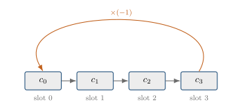
**Figure 4.1.** Multiplying \(c(x)=c_0+c_1x+c_2x^2+c_3x^3\) by \(x\) inside \(R_q=\mathbb{Z}_q[x]/(x^n+1)\) shifts every coefficient one slot to the right, shown here for \(n=4\) (blue arrows). The coefficient that falls off the top does not simply reappear: it comes back into slot \(0\) *negated* (orange arrow), because the defining relation of the ring is \(x^n=-1\). Concretely, \(x\cdot c(x) = -c_3 + c_0x + c_1x^2 + c_2x^3\). This negacyclic wrap-around, rather than a plain cyclic shift, is the single most important structural fact about ring-based lattice cryptography, and it is exactly the sign flip implemented in Algorithm 3.

Carrying the sign flip through a full product gives the negacyclic convolution: the coefficients of \(c(x)=a(x)b(x) \bmod (x^n+1)\) are \[c_k = \sum_{i+j=k} a_i b_j \;-\; \sum_{i+j=k+n} a_i b_j,\] the ordinary convolution minus the part that has wrapped past degree \(n-1\). Algorithm 3 is the direct schoolbook realisation.

Input: Coefficient arrays \(a_0,\dots,a_{n-1}\) and \(b_0,\dots,b_{n-1}\) of \(a(x),b(x)\in R_q=\mathbb{Z}_q[x]/(x^n+1)\)

Output: Coefficients \(c_0,\dots,c_{n-1}\) of \(c(x)=a(x)b(x)\bmod(x^n+1)\)

1:\(c_0,\dots,c_{n-1} \gets 0,\dots,0\)

2:for \(i = 0,\dots,n-1\) do

3:for \(j = 0,\dots,n-1\) do

4:\(k \gets i+j\)

5:if \(k < n\) then

6:\(c_k \gets c_k + a_i b_j\)▷ ordinary term, degree stays below \(n\)

7:else

8:\(c_{k-n} \gets c_{k-n} - a_i b_j\)▷ wraps past degree \(n-1\): negated, since \(x^n=-1\)

9:end if

10:end for

11:end for

12:return \((c_0,\dots,c_{n-1}) \bmod q\)

Algorithm 3. Polynomial Multiplication modulo \(x^n+1\)

4.9Splitting modulo \(q\): the door to the NTT#

Over \(\mathbb{Q}\) the modulus is irreducible, but over \(\mathbb{Z}_q\) it need not be, and we want it to factor.

Proposition 4.10 (Full splitting). If \(2n \mid q-1\), then \(\mathbb{F}_q\) contains a primitive \(2n\)-th root of unity, \(x^n+1\) splits into \(n\) distinct linear factors over \(\mathbb{F}_q\), and the Chinese Remainder Theorem gives a ring isomorphism \[\mathbb{Z}_q[x]/(x^n+1) \;\cong\; \mathbb{F}_q \times \cdots \times \mathbb{F}_q \quad (n\text{ copies}).\]

Under this isomorphism, multiplication of polynomials becomes coordinatewise multiplication of \(n\) scalars – an \(O(n)\) operation once the map is applied. The map itself, and its inverse, are computed in \(O(n\log n)\) by the NTT (Chapter 6); that is the entire reason the NTT exists.

Remark 1.1 (Kyber’s partial split). Kyber uses \(q=3329\) and \(n=256\), and \(q-1 = 3328 = 2^8\cdot 13\). Here \(n=2^8\) divides \(q-1\) but \(2n=2^9\) does not, so \(\mathbb{F}_q\) has a primitive \(256\)-th root of unity but no primitive \(512\)-th root. Consequently \(x^{256}+1\) does not split completely; it factors into \(128\) irreducible quadratics, and Kyber’s NTT maps \(R_q\) to \(128\) copies of \(\mathbb{F}_q[x]/(\text{quadratic})\) rather than to \(256\) scalars. The principle is identical – CRT turns one multiplication into many independent small ones – only the block size differs.

4.10RLWE as structured LWE#

With the ring in hand, the transition from LWE to RLWE is a change of alphabet: \[\underbrace{A\mathbf{s}+\mathbf{e}=\mathbf{b}}_{\text{LWE, over } \mathbb{F}_q^n} \qquad\longrightarrow\qquad \underbrace{a(x)\,s(x)+e(x)=b(x)}_{\text{RLWE, over } R_q}.\] The random matrix \(A\) is replaced by structured polynomial multiplication, because one polynomial encodes an entire negacyclic linear map; the secret and error become polynomials. This can substantially reduce storage relative to an unstructured matrix, but there is no parameter-independent “factor of \(n\)” size theorem: a comparison depends on dimensions, sample counts, moduli, security targets, and encoding. The precise RLWE construction is the subject of Chapter 12.

4.11Experiments#

R.<x> = PolynomialRing(GF(17))
S.<y> = R.quotient(x^4 + 1)

# 1. the quotient relation and its powers
print(y^4, y^5, y^8)          # -1, -y, 1

# 2. negacyclic wrap-around by hand: multiply by y
c = 2 + 3*y + 4*y^2 + 5*y^3
print(y * c)                   # top coeff returns to slot 0 negated

# 3. a quotient element is a length-4 coefficient vector
print((3*y^3 + y + 2).lift().list())

4.12Summary#

This chapter built the ring \[R_q = \mathbb{Z}_q[x]/(x^n+1)\] from the ground up: a polynomial ring \(\mathbb{F}_q[x]\), made finite by quotienting out the ideal \((x^n+1)\), whose elements are length-\(n\) coefficient vectors and whose multiplication is negacyclic convolution. Choosing \(n\) a power of two makes the modulus a cyclotomic polynomial with excellent structure, and choosing \(q\) so that the modulus splits mod \(q\) opens the door to the NTT. The next chapter, Lattices, turns from this algebraic view to the geometric one, where the hardness of the underlying problems actually lives.